SlideShare a Scribd company logo
Pergamon
Transpn. Res.-B.Vol. 29B,No. 3, pp. 155-170.1995
Copyright0 1995ElscvierScienceLtd
Printed in Great Britain.Allrightsreserved
0191-2615/95
$9.50 + .OO
0191-2615(94)00024-7 zyxwvutsrqponmlkjihgfedcbaZYXWVU
A MODEL FOR THE DYNAMIC SYSTEM OPTIMUM
TRAFFIC ASSIGNMENT PROBLEM
M. 0. GHALI and M. J. SMITH
Department of Mathematics, University of York, York YOl 5DD, England zyxwvutsrqponmlkjih
(Received 13 November 1992; in revisedform 17 May 1994)
Abstract-We describe a deterministic queueing assignment model which seeks to reduce total
travel delays in a road traffic network by routeing drivers according to the total delay caused on
each link (the local marginal delay). The model is approximate and is applicable to networks with
many origin-destination pairs and many bottlenecks. Optimality of the solution determined by the
model is discussed. It is particularly shown that, unlike in the steady state (Dafermos and Spar-
row, 1%9), reducing total travel times by using the local marginal delay will not generally result
in an optimal solution. Results are provided for two networks.
1. INTRODUCTION
The dynamic system optimum traffic assignment problem is the problem of determining
time-varying link flows in a congested road network where drivers are assumed to be
cooperative in minimising total transportation delays. It is an essential tool in modeling
peak periods for three reasons: ( 1) It indicates the best network performance when
drivers are guided by a central controller, given that guidance is accepted; (2) it could be
used as a planning tool in a traffic management study to assess how far a user-optimised
flow pattern may be inefficient from the community point of view as a whole and (3) it is
useful for estimating the road prices which internalise the externalities of congestion,
accidents and environmental impacts. Yet most of the work done up to date on this
problem has been confined to a single commodity network, where all road users in the
traffic network have a single destination.
In this article we describe a model which can be applied to (multi-commodity)
networks with many origins and many destinations. The model considered depends on a
certain link model which differs from other dynamic assignment models in the transporta-
tion literature. Throughout this article, departure times are supposed fixed and given;
and the central articles concerning this case is Merchant and Nemhauser (1978a, b). As
we have already indicated, their link model is different from the one adopted here;
although their link output function could probably be chosen to coincide with ours.
Perhaps the main difference between the two approaches is that we consider many origins
and many destinations, whereas Merchant and Nemhauser confine themselves to a single
destination.
A number of studies have been triggered by the Merchant and Nemhauser (M-N)
model. Carey (1986, 1987) has tackled the inherent nonconvexity of the M-N model by
introducing flow control and has pointed to the central difficulty of writing down con-
straints which represent the natural first-in, first-out (FIFO) queue discipline. The FIFO
constraint becomes an important issue as soon as there are several commodities and
dynamics. Friesz et al. (1989) have also studied the M-N model, but in a time-continuous
setting, utilising the Kuhn-Tucker optimality conditions at the solution. However, the
essential difficulties of this natural and general case (FIFO, and nonzero flow controls
perhaps) are not tackled and remain unresolved.
Nonzero flow controls arise in a multi-commodity network for it may sometimes be
beneficial to hold, at a bottleneck, traffic traveling to a certain destination while other
traffic traveling to a different destination should be let go. Though beneficial, nonzero
1.55
156 M.O. GHALI andM.J. SMITH
flow controls may not always be attainable. To show that, an example of nonzero flow
controls is given in Appendix A.
The model of this article guarantees zero flow control or no holding back of traffic
and the first-in, first-out queue discipline at each bottleneck using simulation. The use of
simulation allows us to take the usual behaviour of drivers as given; if a vehicle at a
priority junction is on the main stream, then it is undelayed, whereas it is delayed on the
minor stream until it is able to join the main stream, as would happen in real life. Thus
the traffic assignment ensuing the application of our model is an assignment in which
holding back does not occur and in which vehicles exit the queues at bottlenecks in exactly
the same way that they joined.
In the model the study period is discretised into a number of time slices during each
of which link attributes, such as entry flow rates and exit flow rates from each link, are
assumed to be constant. The model treats vehicles as indivisible entities and assigns each
vehicle a single route, connecting the appropriate origin-destination pair. Routes, once
determined, are remembered.
The overall model has two basic parts: ( 1) a network loading procedure, and (2) a
reassignment procedure. These two basic parts are interleaved in the overall model to
reduce total travel delays in a road network. The purpose of the network loading proce-
dure is (1) to simulate the interaction between vehicles (on links and possibly at junc-
tions), (2) to calculate the entry flow into each link for a given set of route inflows and
(3) to evaluate network performance. The reassignment procedure is concerned with the
calculation of the vehicles’ routes. The chosen routes for each vehicle correspond to the
cheapest route when ordinary link costs are replaced by local marginal costs or delays.
The article is organised as follows. Section 2 gives the modeling assumptions made.
Section 3 is concerned with certain details of the model proposed here. Section 4 provides
numerical results for two network tests obtained by implementing the model presented in
Section 3. Section 5 provides some discussion and indicates some limitations of the model
presented here. Finally, Section 6 concludes the article.
2. MODELlNG FRAMEWORK
In this article we regard travel costs equivalent to real travel times, and we hold that
real travel times are a combination of queueing delays and running, or rolling, travel
times. We do not make a distinction between time spent queueing and time spent rolling.
2.1. zyxwvutsrqponmlkjihgfedcbaZYXWVUTSRQPONMLKJIHGFEDCBA
The network
As usual, the network consists of links, junctions, origins and destinations. Vehicles
enter the network at origins and leave the network at destinations. Origins are connected
to destinations through links, which themselves are connected through intermediate junc-
tions. Links represent real carriageways in the original network and can have differing
properties, such as number of lanes, capacities, etc. Junctions in the network can be
controlled or uncontrolled, and the intersecting movements at junctions are supposed
here to be able to filter through one another with no added delay. This may not be truly
representative of the actual traffic movements at junctions, but we make this simplifying
assumption here for ease of presentation.
2.2. Traffic demand
Traffic demand is represented by a set of indivisible vehicles which leave the origins
at predetermined and fixed times. Accordingly, we view traffic demand as inelastic and
times of departure as fixed. The vehicles leaving the origins are each assigned a single
route; thus we do not allow for splitting of vehicles while these vehicles proceed to their
destinations.
2.3. The link model
We shall suppose that link carriageways have associated exit bottlenecks, each of
capacity w. We shall also suppose that each link has an associated travel time which is
equal to the time needed to traverse the link itself when uncongested.
Dynamic system optimum traffic assignment 157
2.4. zyxwvutsrqponmlkjihgfedcbaZYXWVUTSRQPONMLKJIHGFEDCBA
Flow into the link
Given the route of each vehicle, and remembering that we discretise the study period
into a number of time slices, for each link the total link entry flow during a certain time
slice is the number of vehicles entering that link during that certain time slice. The link
entry flow rate during a time slice is determined by dividing the total number of vehicles
entering the link during the time slice by the duration of the time slice.
In the steady state, link inflows can be determined easily given route inflows. In the
dynamic case, this is not straightforward because the time dimension affects the order of
vehicles’ entry into each link. In Appendix B, we describe a procedure for determining
link inflows from route inflows. This procedure moves vehicles along their assigned
routes forward in time and respects the order of entry and exit of vehicles from each link.
2.5. Bottleneck queues and delays and link delays
Throughout this article we shall propose that queueing on links is deterministic. By
this we mean that a queue forms on a link during the peak period due to excess entry flow
into the link bottleneck as compared to its service rate w. Further, if the entry flow into
the bottleneck during the peak period is equal to (or less than) the capacity of the
bottleneck, then we assume zero queue.
Figure 1 shows the bottleneck queue profile of a link bottleneck over a number of
time slices. V(t) represents the cumulative entry flow into the bottleneck, and W(t)
represents the cumulative departures from the bottleneck. q(t) and d(t) are the queue
length delay at time t, respectively.
The piecewise-linear cumulative entry flow V(t) in Fig. 1 is an approximation to the
smooth curve V(t) in Fig. 2 and is determined from the link entry flow rate as follows.
(The link entry flow rate is itself determined as described earlier.) For a known link entry
flow rate during each time slice, the total bottleneck entry flow into the bottleneck during
a time slice is determined from the number of vehicles which arrive at the bottleneck
during the time slice; and the bottleneck entry flow rate (v in Fig. 1) is just the total
number of vehicles divided by the time slice duration.
In algebraic terms, the cumulative V(t) and W(t) of the bottleneck queue profile in
a time slice (say) i, are (when there is a queue throughout the time slice).
V(ti) = Vj * (ti - t,-i) + V(t,_])* (1)
Fig. 1. Linear approximation to bottleneck queue profile q( ).
158 M.O.GHALI andM.J. SMITH
v,w
t
Fig. 2. Queue length q = q(f) and weueing delays d = d(t) at a link bottleneck.
W(ti) = W ’ (tj - ti-I) + w(ti-I)> (2)
where (ti - ti_, ) is the duration of time slice zyxwvutsrqponmlkjihgfedcbaZYXWVUTSRQP
i, Viis the bottleneck entry flow rate during
time slice i and w is the departure rate from the bottleneck. Note that the bottleneck entry
flow rate, or the slope Vi,is constant during each time slice, and w is time independent,
because we assumed that the bottleneck capacities are fixed throughout the study period.
The area confined between the two curves, I/ and W in Fig. 1, represents the total
queuing delays of all drivers entering the link. The link delay encountered by each vehicle
entering a link is supposed to be the sum of ( 1) a flow-independent or uncongested travel
time needed to arrive at the link bottleneck, and (2) the queueing delay encountered at
the bottleneck on arriving at the bottleneck at time t. The queueing delay d(t) at time t is
calculated using the relation d(t) = q( t)/w, where q is the queue length at time 1.
2.6. The local marginal delay (LMD)
The marginal delay arising from a single vehicle entering a certain link can be viewed
as the sum of ( 1) the link delay encountered by the single vehicle itself (as before), and
(2) the additional delay experienced on that link, at the bottleneck, by every vehicle
arriving between time t and T, due to the single vehicle arriving at the bottleneck at time
t. (Here T is the time at which the cumulative departure and arrival curves meet, or the
time at which the queue at the bottleneck disappears. )
The additional delay imposed by the single vehicle on others (on the same link) is
M - d, where rn, as shown in Fig. 3, is the difference between T and the time t at which
the single vehicle arrives at the bottleneck. To explain how this is obtained, Fig. 3 shows
the arrival of a unit vehicle (size = 1) at time t3, whose presence induces additional delay
to the overall queueing delays on the link by an amount that is equivalent to the solid area
in Fig. 3. Now the solid area is equal to the horizontal area in Fig. 3, which is
(the horizontal distance m) x (unit vehicle size),
or just m (because the unit vehicle is one). But part of m is the link delay, d, encountered
by the single vehicle. Thus the additional delay imposed on others is m - d.
Dynamic system optimum traffic assignment 159
v.w
Local marginal delay
equals this area,
which equals zyxwvutsrqponmlkjihgfedcbaZYXWVUTSRQPONM
thisarea. zyxwvutsrqponmlkjihgfedcbaZYXWVUTSRQPONML
4 t?_ t3 t4 T
Fig. 3. Local marginal delay m( tP) at a bottleneck.
3. AN ALGORITHM FOR THE DYNAMIC TRAFFIC ASSIGNMENT PROBLEM
The algorithm considers one vehicle at a time and performs two basic operations for
each of the vehicles. These operations are ( 1) reroute each single vehicle in the light of
current marginal delays, and (2) load the network so that a check can be made to
determine if the rerouting of the single vehicle reduces total travel delays. These two
operations are repeated for all vehicles, time and time again, until no more new routes are
allocated.
Next we detail the overall algorithm which combines the aforementioned two opera-
tions. We leave its precise form for Appendix C. For loading the network, Appendix B
describes a loading procedure. A feature of this loading procedure is that it implicitly
ensures that the natural FIFO queue discipline and no holding back of traffic at bottle-
necks are both satisfied while evaluating network performance.
3. I. The main steps of the algorithm
These steps are iteratively performed:
1. Start from any initial route pattern which prescribes a route for each vehicle. Load the
network to obtain the link inflow pattern corresponding to the initial route pattern,
and determine the resulting total travel delays.
2. This step is repeated for all vehicles sequentially. For each vehicle in turn,
a. Determine the vehicle’s new route according to the local marginal delay of each link.
b. Determine new value of total travel delays due to the vehicle’s new route. If the new
route reduces total travel delays, then accept new route. If not, then retain the
vehicle’s old route.
3. If new routes were allocated in step 2, or total travel delays were reduced, then go to
step 2 for another iteration. Otherwise, terminate.
3.2. The purpose of each step
Step 1. To reroute we need to have the network already loaded. So an initial route
set which prescribes a route for each vehicle should be chosen. This can be the set of
routes based on cheapest routes using uncongested (flow-independent, zero queueing)
link travel times. (The loading of the network can then be achieved by using the method
described in Appendix B. )
160 M.O.GHALI andM.J. SMITH
Step 2. This step reroutes each individual vehicle according to the local marginal
delay of each link and ensures that only descent directions are chosen. For each vehicle
being considered, the vehicle is first rerouted (step 2a), whereas all other vehicles’ routes
are fixed, and second the outcome of rerouting the vehicle is determined in step 2b.
Step 2~. The route of each vehicle is determined here using a nonlabel setting mini-
mum route search routine, such as the Bellman-Ford (Bellman, 1958) routine. A label
setting routine, such as that due to Dijkstra (1959), is difficult to employ in a dynamical
setting such as this. This is because the arc length of each link can vary with time, so to
consider the various possibilities a nonlabel setting routine is required. An example in
which Dijkstra’s routine fails to calculate the (marginal delay) shortest route is given in
Ghali and Smith (1993).
In using the Bellman-Ford routine in this context, the arc length of each link is the
local marginal delay, but the times of exit into and entry from each link correspond to the
times when the vehicle actually enters and leaves each link. Accordingly, two labels need
to be employed for performing the shortest route calculation of each vehicle with respect
to the local marginal delays. One of these labels remembers the route (marginal) delays
from the origin to every node considered while branching out from the origin, whereas
the other remembers the travel times. We refer to the former as the marginal delay label
and the latter as the time label.
Due to the dynamical aspect of the problem, the local marginal delay of each link
can be different for different times, even within each time slice of the study period. These,
however, need not be calculated beforehand for all links and for all times. Each time a
vehicle’s route is calculated, the marginal delay of each link can be computed while the
shortest route routine is in operation. This is done by keeping track of the vehicle’s time
of entry into each link and the time of arrival at each bottleneck (using the time label),
while the routine branches out from the origin node of the vehicle to label (using the
marginal delay label) the other nodes with the marginal delays. For instance, on arrival at
a certain link bottleneck at a certain time, the routine determines the marginal delay, in
addition to the time to exit from that certain bottleneck at that certain time, using the
bottleneck queue profile, such as in Fig. 1. With the time to exit from that certain
bottleneck now determined, the time of entry into downstream links and the time of
arrival at the downstream bottlenecks of these links thus become known for calculating
the marginal delays at the downstream bottlenecks.
Step 2b. In this step the network is loaded to evaluate network performance. When
loading the network, the route of the vehicle being considered is the one calculated in step
2a while all the other vehicles are kept on their current routes.
This step has a principal role in the algorithm. It allows us to prove convergence of
the algorithm by checking on whether the new route calculated with respect to the local
marginal delays is a descent direction. If so, step 2b allows for route swapping or move-
ment along that direction. Otherwise, no route swapping is allowed.
The reason a check needs to be made on the total travel delays is because, as we will
see later, route marginal delays based on the local marginal delay of each link along the
route are not necessarily descent directions. Thus, by making such a check in this step,
only descent directions are chosen; directions which are not so are rejected by retaining
the vehicle on its previous route.
Step 3. The purpose of this step is to call for another iteration by restarting the
algorithm execution from step 2 if the total travel delays were reduced in the current
iteration. Obviously, the algorithm terminates when no total travel delay reduction oc-
curred in the current iteration.
3.3. Convergence of the algorithm
The overall algorithm is said to converge if ( 1) the loading procedure used converges,
(2) the shortest route routine used converges and (3) the structure of the algorithm itself
converges. As far as the loading procedure is concerned, we use the time-slice-by-time-
slice loading procedure described in Appendix B. This is once through and goes forward
Dynamic system optimum traffic assignment 161
in time to determine the link flows corresponding to the vehicles’ predetermined (loop-
free) routes. Hence, it stops when all the vehicles have arrived at their destinations. The
vehicles’ routes are loop free because the arc length is always positive; neither the delay
inflicted by one vehicle on others on the same link nor the uncongested link travel time
can be negative. As for the shortest route routine used, this, as we mentioned earlier, is
due to Bellman-Ford (Bellman, 1958). This routine is known to converge after at most
N - 1 iterations, where N is the number of nodes in the network.
It remains to show the convergence of the structure of the algorithm. The algorithm
is guaranteed to converge for the obvious reasons: ( 1) The (total travel delay) objective
function is bounded from below (total travel delays cannot be less than zero), and (2) the
objective function monotonically decreases in the order C’ > Cz > . . . > C’-’ = C’,
from iteration 1 to i - 1 because, within each iteration, the spatial rerouteing of each
vehicle is checked (in step 2b) and allowed only if it decrements the total travel delays.
The algorithm finally stops when the total travel delays cannot be further reduced from
rerouting any vehicle. This is in iteration i.
Although the structure of the algorithm is shown to have a limit point, the limit point
may not necessarily be the optimal solution because (1) route marginal delays based on
the local marginal delay of each link on the route are not necessarily descent directions
(see Section 5), and (2) the dynamic system optimum problem is a nonconvex problem
(see Ghali and Smith, 1993).
4. zyxwvutsrqponmlkjihgfedcbaZYXWVUTSRQPONMLKJIHGFEDC
SOME COMPUTATIONAL EXPERIENCE
To provide some computational results, two networks were considered. For each
network, we compare network performance due to routing vehicles according to their link
local marginal delays as opposed to the performance resulting from vehicles follow-
ing their own cheapest routes, which would normally be chosen by each vehicle/driver on
the basis of link delays, without taking into account the delays imposed on others. The
pattern of flow resulting from each driver following its cheapest route in that sense is
commonly known as user equilibrium. We imitate this here using the algorithm specified
in Appendix D. This is basically similar to the algorithm which routes vehicles on the
basis of the local marginal delay except that ( 1) the vehicles’ link travel delays are, in this
case, the link delays defined in Section 2, and (2) no monitoring of the total travel delays
is performed; the algorithm stops when no route swap occurs in some iteration.
In solving for a user equilibrium, as in Appendix D, we cannot guarantee a proof of
convergence, mainly because of the following. The user equilibrium problem is currently
under considerable research, and currently there is no proof that a user equilibrium exists
when the natural FlFO is imposed at the link bottlenecks and when the link model is the
one adopted in this article. Currently, there is no theoretically sound and proven proce-
dure which can be used to determine a user equilibrium flow pattern. For more discussion
on the difficulties with the user equilibrium problem, see Smith and Ghali (1990), Smith
( 1993), Addison and Heydecker ( 1990) and Bernstein et al. ( 1993).
Curve LMD in Figs. 5 and 6 shows network performance due to routing drivers
according to the local marginal delay, whereas UE is due to the estimated user equilib-
rium.
The results given next were obtained using the computer program RONETS (Road
NETwork Simulator). RONETS is a fast developing, multi-purpose, dynamic traffic
simulator.
4. I. zyxwvutsrqponmlkjihgfedcbaZYXWVUTSRQPONMLKJIHGFEDCBA
Network 1
This network is shown in Fig. 4. It is taken from Allsop and Charlesworth, (1977).
The results for this network are summarised in Fig. 5. This shows that (for this network)
substantial benefits accrue from routing vehicles according to the local marginal delay of
162 M.O. GHALI andM.J. SMITH
Fig. 4. Geometry of Network 1.
each link rather than the user equilibrium. Total travel delays are reduced by about 20%.
Only two iterations were needed for the LMD solution. The UE solution was observed
after five iterations.
4.2. zyxwvutsrqponmlkjihgfedcbaZYXWVUTSRQPONMLKJIHGFEDCBA
Network 2
This network represents a town in England. It has 250 links and 50 junctions. The
results in Fig. 6 show that network performance corresponding to LMD is better than the
performance corresponding to UE; total travel delays are reduced by about 3%. Four
iterations were needed for the LMD solution. The UE solution was observed after eight
iterations.
RONETSresults for the network in Allsop (1977)
27000
26000
25ooo
B
‘n 24000
23000
._
2 3 4 5
Iteration
Fig, 5. Performance of Network 1under user equilibrium and local marginal delay assignment.
Dynamic system optimum traffic assignment 163
RONETS results for a town in England (250 links, 50 junctions)
555000 , a I I I
550000
530000
525000 zyxwvutsrqponmlkjihgfedcbaZYXWVUTSRQPONMLKJIHGFEDCBA
0 1 2 3 4 5 6 I 8
Iteration
Fig. 6. Performance of Network 2 under user equilibrium and local marginal delay assignment.
5. THE OPTIMALITY OF THE SOLUTION OF THE MODEL
The ability of the method to deal with many origin-destination and many bottleneck
networks in a dynamic context has been demonstrated in the network tests provided. The
method, on the other hand, is approximate, and as such it may not produce an optimal
solution. The method is approximate due to the following limitations of the local mar-
ginal delay, viewed on a route level:
1. Route marginal delays based on the local marginal delay of each link along the route
do not necessarily determine the steepest descent direction.
2. Route marginal delays based on the local marginal delay of each link along the route
do not necessarily determine a descent direction, at all.
We will not address in this article issues relating to uniqueness, convexity/noncon-
vexity and differentiability of the model presented here. These have recently been ad-
dressed in Ghali and Smith (1993), where it is particularly shown that the dynamic system
optimum problem may generally not have a unique solution and may be a nonconvex and
nondifferentiable problem. Also in Ghali and Smith (1993) a different marginal delay
system, overcoming some of the shortcomings of the marginal delay system of this article,
is described. (An algorithm based on this different marginal delay system is presented in
Ghali and Smith, 1992.)
Next, we explain the limitations of the local marginal delay. zyxwvutsrqponmlkjihgfedcbaZ
5. I. Route marginal delays, based on LMD, do not necessarily determine the steepest
descent direction
The model considers only the local marginal delay of each link while rerouting each
vehicle. In the steady state, rerouting vehicles along the routes which have least link
(local) marginal delay determines the least costly pattern of flow (if the total delay
function is convex; see Dafermos and Sparrow, 1969). Regrettably, this feature does not
carry over to the dynamic state. This is so because route marginal delays, based on adding
the local marginal delay of each link along the route, do not be always global, except for
some network topologies.
To show that route marginal delay may not always determine the steepest descent
direction, we consider the network shown in Fig. 7. This is similar to the network consid-
ered in Appendix A and shown in Fig. 8. Here it is modified slightly to allow for route
164 M.O. GHALI andM.J. SMITH
Fig. 7. Network showing two route choices for commodity 02 = D2.
choice between 02 to D2 by adding the route 02-5-6-D2. Traveling time on route 02-5-
6-D2 is assumed to be equal to 6 seconds. Travel times on other links, bottleneck capaci-
ties and commodity demands are as in Appendix A.
For this example, the optimality of the solution based on link-local marginal delays,
and as obtained by our model, will depend on the value of 6. Because we are interested in
establishing that route marginal delays do not necessarily determine the steepest descent
direction, we will take a value for 6 which shows this clearly. The chosen value of 6 is 125
seconds. This value is greater than the largest value of the marginal delays at bottleneck
Bl, which is 120 seconds. This value of 120 seconds corresponds to the case in which all
the flow of commodity 2 travels through Bl; in this case the queue dissipates at Bl at time
120 seconds and the total travel delays are 121,500, as in Appendix A.
Now consider swapping some of the flow rate from commodity 2 to take the route
02-5-6-D3. Let the swap value be Eveh/sec, out of the total demand 10veh/sec. The total
travel delays (networkwide) then become
180 x (E - 10) x (-27,000 + 2000~ - 50~~ + E~)/( -20 + e)* + 7500~ (3)
and the gradient of the total travel delays, with respect to E, is
300 x (200,000 - 26,500~ + 1800~’ - 70C3 + E4)/( -20 + E)3 + 7500. (4)
For E = 0, the total travel delays are, as before, 121,500 veh/sec, and the gradient is
equal to - 1500, which is negative. So the networkwide travel delays can be reduced by
swapping some of the flow of commodity 2 from route 02-5-6-D2 to route 02-5-6-D2 (or
by moving in the direction of positive values of E, from the bottom to the top route).
However, with the value of 6 being 125 seconds and the largest value of the local
marginal delays at Bl being 120 seconds, no traffic from commodity 2 will be forced to
take route 02-5-6-D3 when routing traffic from commodity 2 according to these marginal
delays, because the local marginal delay at Bl ( = 120) is less than 6 ( = 125) on route
02-5-6-D2.
Fig. 8. An example network with three commodities and two bottlenecks.
Dynamic system optimum traffic assignment 165
In view of this example, the model does not in general determine a system optimum
pattern of flow. Nonetheless, in the single-bottleneck-per-route case, our algorithm can
be guaranteed to determine the system optimal pattern of flow. This single-bottleneck
case is introduced in Smith and Ghali (1990) and corresponds to a network in which each
reasonable route connecting each origin-destination pair in the network passes through
no more than a single active bottleneck.
5.2. zyxwvutsrqponmlkjihgfedcbaZYXWVUTSRQPONMLKJIHGFEDCBA
Route marginal delays, based on LMD, do not necessarily determine a descent
direction, at all
Here we show that route marginal delays based on link-local marginal delays may
not always determine a descent direction, We consider the preceding example again, but
here we assume that initially all the flow of commodity 2 is on route 02-5-6-D2. In this
case total travel delays from eqn (3) are 75,000, and no queues exist at bottleneck Bl.
Because no queues now exist, the marginal delay at Bl is thus equal to zero, which is
considerably less than the value of 6. So the route marginal delays along route 02-l-3-D2
(having a zero value) are less than those along route 02-5-6-D2 (having a value of S). In
spite of that, moving some of the flow of commodity 2 in the direction from the top route
to the bottom route increases the total travel delays, because the gradient in eqn (4) at E
= 10 is positive in this direction. Hence, the route marginal delays are not pointing in the
direction which reduces the total travel delays.
6. CONCLUSIONS AND FURTHER WORK
This article presented a model for approximately solving the dynamic system opti-
mum problem; the model is based on the local marginal delay of each link. We have also
shown that the local marginal delay has two limitations-namely, that in contrast with
the steady state, route marginal delays based on adding up the local marginal delay of
each link do not necessarily determine the steepest direction nor do they necessarily
determine a descent direction in the dynamic state. Results for two networks were given.
These show that there are benefits from routing vehicles according to the local marginal
delay, in spite of the aforementioned limitations. Finally, Appendix B described a net-
work loading procedure. This may prove useful in other related topics, such as route
guidance and equilibrium problems.
The work in this article may be extended in a number of ways. For instance, consider
the computational issue. The computational effort needed to determine the solution of
the model may be reduced by constructing a different version of the algorithm which
may be implemented on a parallel machine. Similarly, the network loading procedure
computational time may also be reduced by implementing it on a parallel machine.
In a different direction, it would be interesting to design a procedure which deter-
mines the road prices corresponding to the local marginal delay system presented in this
article. The local marginal delay cannot be directly translated into efficient road prices,
because the intention of the marginal delay is to influence route choice in this article. For
example, consider a single-link-bottleneck network that has a travel demand exceeding
the capacity of the bottleneck during the rush hour. Here there is no route choice;
however, the local marginal delay for a vehicle arriving at the bottleneck at the beginning
of the rush hour can be substantial because it corresponds to the difference between the
time the vehicle arrives and the time at which the queue at the bottleneck ceases to exist.
But if we were only concerned with route choice to reduce congestion, the road prices
should be zero. Thus, this is not equal to the (large) marginal delays at this link bottle-
neck.
Acknowledgements-The authors would like to express their gratitude for the many valuable comments made
by an anonymous referee on an earlier version of this article. The work reported here has been partly funded by
the Science and Engineering Research Council of the United Kingdom.
166 M.O. GHALI andM.J. SMITH
REFERENCES
Addison, J. D., & Heydecker, B. ( 1993). A mathematical model for dynamic traffic assignment. In C. Daganzo
(Ed.), zyxwvutsrqponmlkjihgfedcbaZYXWVUTSRQPONMLKJIHGFEDCBA
Proceedings of the 12th International Symposium on Transportation and Traffic Theory (pp. 171-
184). New York: Elsevier.
Allsop, R. E., & Charlesworth, J. A. (1977). Traffic in a signal-controlled road network: An example of
different timings inducing different routings. Traffic Engineering and Control, 18, 262-264.
Bellman, R. E. (1958). On a routing problem. Quart. Appl. Math., 26, 87-90.
Bernstein, D., Friesz, T. L., Tobin, R. L., & Wie, B-W. (1993). A variational control formulation of the
simultaneous route and departure-time choice equilibrium problem. In C. Daganzo (Ed.), Proceedings
of the 12th International Symposium on Transportation and Traffic Theory (pp. 107-126). New York:
Elsevier.
Carey, M. (1986). A constraint qualification for a dynamic traffic assignment model. Transportation Science,
20(l), 55-58.
Carey, M. (1987). Optimal time-varying flows on congested networks. Operations Research, 35(l), 58-69.
Dafermos, S. C., & Sparrow, F. T. (1969). The traffic assignment problem for a general network. J. Res. Nat.
Bureau of Standards-B MathematicalSciences, 73B(2), 91-I 18.
Dijkstra, E. W. (1959). A note on two problems in connexion with graphs. Numerische Mathematik, 1, 269-
271.
Friesz, T. L., Luque, F. J., Tobin, R. L., & Wie, B. W. (1989). Dynamic network traffic assignment considered
as a continuous time optimal problem. Operations Research, 35, 58-69.
Ghali, M. O., & Smith, M. J. (1992). Approximation to optimal dynamic traffic assignment of peak period
traffic to a congested city network. Paper presented at the 2nd International Capri Seminar on Urban Traffic
Networks, Capri, Italy, July 5-8.
Ghali, M. O., & Smith, M. J. (1993). Traffic assignment, traffic control and road pricing. In C. Daganzo
(Ed.), Proceedings of the 12th International Symposium on Transportation and Traffic Theory (pp. 147-
170). New York: Elsevier.
Merchant, D. K., & Nemhauser, Cl. L. (1978a). A model and an algorithm for the dynamic traffic assignment
problem. Transportation Science, I2( 3), 183-199.
Merchant, D. K., & Nemhauser, G. L. (1978b). Optimality conditions for a dynamic traffic assignment model.
Transportation Science, I2( 3), 200-207.
Smith, M. J. (1993). A new dynamic traffic model and the existence and calculation of dynamic user equilibria
on congested capacity-constrained road networks. Transportation Research, 27B( I). 49-63.
Smith, M. J., & Ghali, M. 0. (1990). Dynamic traffic assignment and dynamic traffic control. In M. Koshi
(Ed.), Proceedings of the Ilth International Symposium on Transportation and Traffic Theory (pp. 273-
290). New York: Elsevier.
APPENDIX A: FLOW CONTROLS IN A MULTI-COMMODITY NETWORK:
AN EXAMPLE
Consider the network shown in Fig. 8. In this network, three commodities are observed, commodity 1
corresponding to the origin-destination pair Ol-Dl, commodity 2 to 02-D2, and commodity 3 to 03-D3. For
simplicity, traveling time on links is taken as zero. Further, the network is assumed to have two bottlenecks; the
first is located at the exit of link l-2, denoted as zyxwvutsrqponmlkjihgfedcbaZYXWVUTSRQPONM
Bl , and the second at the exit of link 3-4, denoted as B2. Each
bottleneck has a capacity of 10veh/sec. The demand from 01 and 02 starts at time t = 0 seconds, at a rate of
10 veh/sec, for a period of 60 seconds. The demand from 03 starts at t = 60 seconds, at a rate of 10 veh/sec,
and continues for 5 hours at this rate.
Now we consider two cases: ( 1) Traffic from commodity 2 is held back at node 1, perhaps by means of a
traffic controller which acts as a flow-control variable in this case; and (2) traffic from commodity 2 merges
with traffic from commodity 1 at node 1.
In the first case, when traffic of commodity 2 is held back at node I, the traffic from commodity 1 could
proceed through the first and second bottlenecks without having to queue at either bottleneck. The total travel
delavs in this case are iust aueueina delays of value 36,ooOveh/sec due to holding the traffic from commodity 2
at node 1. Note that traffic-from commodity 3 in this case passes through the second bottleneck without having
to queue, because all the traffic from commodity 1 would have arrived at its destination by the time traffic from
commodity 3 starts entering the bottleneck.
On the other hand, in the second case, when traffic from commodity 2 merges with traffic from commodity
I, queues at both bottlenecks Bl and B2 then develop. In this case, precisely half the demand from commodity
1 emerging from the first bottleneck Bl would merge with flow from commodity 3, thus increasing the queueing
delay from 36,000 to 121,500 veh/sec, which is a substantial increase in total travel delays.
It is clear, therefore, from this example that the total travel time is reduced if the traffic of commodity 2
was held back at or before node 1. However, in the absence of a control mechanism (e.g. a traffic light at node
I), it is not possible to hold traffic from commodity 2 merging with the traffic from commodity 1 in entering
the bottleneck Bl.
APPENDIX B: A METHOD FOR LOADING THE NETWORK
In the steady state, loading of the network is straightforward. Given the routes and the route flows, the
flow on a link can be calculated by addina all the route flows entering the link. Having found the link flows,the
total network delay can then be readily calculated, perhaps utilising a proper delay function for every link.
In the dynamic state, the aforementioned nicety does not carry over due to the additional time component.
Dynamic system optimum traffic assignment 167
v,w
V(t) of slope vg zyxwvutsrqponmlkjihgfedcbaZYXWVUTSRQPONM
11 k t3
Fig. 9. 3-time slice incomplete queue profile.
To account for this we describe in this section a method which goes forward in time. We call this a time-slice-by-
time-slice loading procedure. The lengths of the time slices in this loading procedure are chosen so that none is
greater than the shortest link (uncongested) travel time in the network. The reason for restricting the time slices
as such is given next.
The lime-slice-by-rime-slice loading procedure
As in the main body of this article, we call the profile depicted in Fig. 1, which expresses the relation
between the entry and exit flow of a particular link bottleneck the queue profile of the link bottleneck. We will
also call a bottleneck queue profile of a bottleneck which is determined up to the end of a certain time slice,
which is not the last time slice of the modeling period, a bottleneck incomplete queue profile.
Figure 9 shows an incomplete queue profile for some link bottleneck determined up to the third time slice;
Fig. 10 shows the same queue profile but with one time slice added; Fig. 1 shows the complete queue profile.
In explaining this loading procedure, we will start from a point at which all the link queue profiles are
calculated and stored up to the end of a certain time slice. [Storing of the queue profile for some link and some
time slice within the planning horizon requires storing the initial queue length at the beginning of the time slice
and the inflow rate into the link within the time slice. Knowledge of these two values enables one to calculate
v,w
V(t) of slope VJ
between t2and ts.
4 tz t3 t
Fig. IO. 4-time slice incomplete queue profile.
168 M.O. GHALI andM.J. SMITH
the queueing delays for any vehicle joining the back of the queue on the link within the time slice. Of course,
this is only because we assumed the inflow rate into each link bottleneck as constant; see eqns (5) and (a).]
Then it is necessary to complete the queue profile of a certain link beyond that certain time slice to account for
the queues in the current time slice and beyond. Following the same argument, it then becomes easy to determine
the queue profile of other links within the same current time slice and for subsequent time slices.
Some of the vehicles within the current time slice will be newly arising from the origin nodes and others will
be continuing to their respective destinations. The effects of these vehicles on the network in regard to the total
delay have yet to be considered before exiting the network. For vehicles which have arrived at their destination
before the current time slice, their effect on the network is assumed to have been considered already and their
total delay calculated, as in the following discussion.
Consider some link I connected to a number of upstream links which feed into link I. Denote the set of the
upstream links as B(I). The arrival rate at the bottleneck of link I for the current time slice, say s, can be made
known from the expression
where fk is the size of vehicle k, and pr - j - I means that ( 1) vehicle k is entering link I from some link j in B(I)
or an origin situated at the beginning of link I, and (2) vehicle k joins the back of the queue at the end of link I
within the current time slice.
Having calculated the arrival rate at the bottleneck of link I within the current time slice, it remains to
calculate ( 1) the delay encountered on link I by each vehicle k; and (2) the delay further downstream, if vehicle
k exits link I in the current time slice and proceeds into a downstream link and joins the back of the queue at the
end of the downstream link within the current time slice. If the vehicle does not arrive at the bottleneck of the
downstream link within the current time slice, its effect is then taken into consideration in the following time
slice. If not, the vehicle would have exited the network at the end of link I. If the vehicle did exit the network,
its route delay is added to the total route delay of all the vehicles which have already left the network.
The queuing delay encountered on link zyxwvutsrqponmlkjihgfedcbaZYXWVUTSRQPONMLKJIHGFEDCBA
I by some vehicle k joining the back of the queue at time tP within
the current time slice can be computed from
(4; + (4 - w,)t%)/w, (6)
where 4: is the queue length at the beginning of the current time slice s and w,is the capacity or the service rate
of link zyxwvutsrqponmlkjihgfedcbaZYXWVUTSRQPONMLKJIHGFEDCBA
I (assumed constant for all time slices).
To calculate the queueing delay further downstream on a do .rstream link, say u, the exit time of each
vehicle from the upstream links, including link I, should be first calculated from expressions such as eqn (6) for
every upstream link connected to U. This means that the queue profiles, up to the end of the current time slice,
of every upstream link connected to link u should have been made known before the queue profile and hence
the total delay of the vehicles entering u can be calculated on link u.
The loading procedure should be performed for each link and for each time slice, but following some
order. In other words, the queue profile of a link within a specified time slice cannot be calculated unless all the
links upstream of this link have had their queue profiles calculated up to the current time slice (or the end of the
previous time slice if the vehicles emerging from the upstream links cannot reach the back of the queue on this
link in the current time slice).
A natural order in calculating the link queue profiles for all the links would be to start first from the origin
nodes. But for a reason that will become obvious later, we require that none of the time slices discretising the
study period into a number of time slices should be greater than the time needed to traverse the shortest link in
the network.
Starting from the origins, in the first time slice, no vehicles will exit any of the links because we assumed
that none of the time slices is larger than the time needed to traverse the shortest link in the network. In this
time slice, all the vehicles which can reach the bottleneck on the links downstream of the origin nodes are
considered in calculating the first time slice of the link queue profiles. Those vehicles which did not reach the
bottleneck are considered as arriving later in a subsequent time slice, and their effects on the link queue profile
has yet to be considered. In the second time slice, all the vehicles which could exit the links on their routes in
the first time slice and could reach the downstream bottlenecks on the downstream links of their routes in
this second time slice are used to calculate the second time-slice part of the link queue profiles on the down-
stream links. In addition, any vehicles which did not reach the bottleneck of the links downstream of the origins
in the first time slice are included in the calculation of the second time slice of the link profiles if they do reach
the bottleneck now. Any newly arising flow from the origins in this second time slice is considered in calculating
the second time-slice part of the link queue profiles of the links downstream of the origin nodes if it reaches the
bottlenecks in this second slice.
After the second slice, the foregoing procedure is repeated until finally, by the end of the last time slice of
the planning horizon, all the links will have had their link queue profiles calculated, all the vehicles will have
arrived at their destinations and the total delay will have been noted.
Next we illustrate why we require that none of the time slices discretising the study period into a number
of time slices should be greater than the time needed to reverse the shortest link in the network.
Consider the network shown in Fig. 1I. In this network we assume that all the turning movements are
permitted and all the routes have positive flows. Suppose we are calculating the nth time-slice part of the queue
urofile of link I. If the nth time slice is too long, the nth time-slice of the queue profile of link I is affected by the
iight-turn flow emerging from link 3, the nth t’lmeslice of the queue profile of link 3 is affected by the right-turn
flow emerging from link 2 and the nth time slice of the queue profile of link 2 is affected by the right-turn flow
emerging from link 1, then the nth time slice of the queue profile of link 1 cannot be calculated. This is like a
deadlock in computer terminology, wherein each process is waiting for the other to finish. However, with a
restriction on the length of each time slice corresponding to the time to traverse the shortest link, this deadlock
Dynamic system optimum traffic assignment 169
Fig. 11.Network with six origin-destination pairs.
does not arise. This is mainly because the nth time-slice part of the queue profile of link I is affected by the
right-turn flow emerging from link 3 in a previous time slice, and so on for links 3 and 2, which are affected by
the flow of a previous of a previous time slice. To put it differently, for the too long nth time slice, the chain-
( 1,nth time slice), (3, nth time slice), (2, nth time slice), ( 1, nth time slice)-is closed if it is read from left to
right to indicate that a (link, time slice) combination is dependent on its adjacent to the right. In this case, both
ends of the chain are interdependent. In contrast, for a sufficiently short time slice, the aforementioned chain
becomes open because both end combinations, although they have a common link (I), would now have different
time slices.
FIFO sutisfied. So far we have discussed how the queue profiles are calculated. We still need to mention
how FIFO is satisfied in the aforementioned loading procedure.
Consider now any two vehicles a and b, joining the back of the queue on some link i within a time slice s.
Suppose that the time vehicle u joins the back of the queue on link j is earlier than the time vehicle b does. Let
the time when vehicle u joins be t: and that of vehicle b be tz. Also, let the time when vehicle a departs from the
queue be tf, and similarly let that of vehicle b to t$. Obviously, tz < t%.It remains to show that tl c tf. If this
relation is satisfied, then we have FIFO.
From eqns (5) and (a), we have for vehicle u
and for vehicle b,
tf = {q’o + (v; - w,)t:}/w, + t:,
1; = {q”o+ (v; - w,)tZ}/w, + 18.
The terms t: and 18can be written in terms of ti and t$ respectively, to get
t: = {w,ti - qi}/vf, and tj = {wti - qi}/vf.
Because tz < t$,this implies
{WY::- q;}/v; < (w,tll - q;}/v;.
After dropping and subtracting common terms, we get
hence FIFO.
The preceding FIFO argument considers only two vehicles within a common time slice. For vehicles
joining the queues in different time slices, a similar construction can be made to show that even then FIFO is
satisfied. We omit this here.
APPENDIX C: AN ALGORITHM BASED ON THE LOCAL MARGINAL DELAY
Notations
p = The number of vehicles constituting the total demand from all origins.
k = A vehicle number or identification.
L = Number of links in network.
r, = Uncongested travel time on link 1.
q: = Queue length in front of vehicle k on link I when joining the back of queue, if any.
w, = Capacity of the bottleneck of link 1.
170 M. 0. GHALI and M. J. SMITH
i = Iteration counter.
p: = Route of vehicle kin iteration zyxwvutsrqponmlkjihgfedcbaZYXWVUTSRQPONMLKJIHG
i.
fk = Size of vehicle k (assumed 1 in this article).
C’ = Total travel costs (or delays) in iteration i, summed up over all vehicles and links. This is the expression:
k=g ,=I.
2 ,2fk(
f/+d/w,)
Steps
1. i = 0.
2. Calculate and store the route of each vehicle which minimises the route delays of the vehicle, based on
uncongested link travel time. Let the route of vehicle k be pi.
3. Calculate total travel delays, C’(using the loading procedure described in Appendix B).
4.Letk=l,i=i+ landC’=C’-‘.
a. Remove vehicle k from each link on route pi-‘. This entails updating the inflow rates into each link and
each link bottleneck on route pi-‘. Only those inflow rates corresponding to the time slices during which
vehicle k enters are updated.
b. Determine new route p: on the basis of the values of m obtained from profiles similar to Fig. 1 for each
link.
c. Assign vehicle zyxwvutsrqponmlkjihgfedcbaZYXWVUTSRQPONMLKJIHGFEDCBA
k to its new route by updating the inflow rates of the corresponding time slices within which
vehicle k enters the links and the link bottlenecks on route p:.
d. Calculate total travel delays TC (using the loading procedure described in Appendix B). If TC < C’, then
the new route of vehicle k is favourable and the old route piv’ is replaced by pi and C’ is made equal to
TC. Otherwise, C’ and p: are left unchanged.
e. If k = p, then go to step 5. Otherwise, increment k by 1 and return to step 4a.
5. If C’ cr C’-‘, return to step 4. Otherwise, the algorithm is terminated.
APPENDIX D: AN ALGORITHM BASED ON LINK TRAVEL DELAYS
The notations are as in Appendix C.
Steps
1. i = 0.
2. Let k = 1, i = i + 1.
a. If i is greater than 1, then remove vehicle k from each link on route p);‘. This entails updating the inflow
rates into each link and each link bottleneck on route pk-‘. Only those inflow rates corresponding to the
time slices during which vehicle k enters are updated.
b. Determine new route pi on the basis of the link delay of each link.
c. Assign vehicle k to its new route by updating the inflow rates of the corresponding time slices within which
vehicle k enters the links and the link bottlenecks on route pi.
d. If k = p, then go to step 3. Otherwise, increment k by 1 and return to step 2a.
3. If new routes were allocated, return to step 2. Otherwise, the algorithm is terminated.

More Related Content

Similar to A Model For The Dynamic System Optimum Traffic Assignment Problem

Effect of mobility models on the performance of multipath routing protocol in...
Effect of mobility models on the performance of multipath routing protocol in...Effect of mobility models on the performance of multipath routing protocol in...
Effect of mobility models on the performance of multipath routing protocol in...
csandit
 
Optimizing IP Networks for Uncertain Demands Using Outbound Traffic Constraints
Optimizing IP Networks for Uncertain Demands Using Outbound Traffic ConstraintsOptimizing IP Networks for Uncertain Demands Using Outbound Traffic Constraints
Optimizing IP Networks for Uncertain Demands Using Outbound Traffic Constraints
EM Legacy
 
CL436 Transport Planning Final Submission
CL436 Transport Planning Final SubmissionCL436 Transport Planning Final Submission
CL436 Transport Planning Final SubmissionGordon Best
 
Vanet report 2020 2nd semester
Vanet report 2020 2nd semesterVanet report 2020 2nd semester
Vanet report 2020 2nd semester
SudarshiniAuradkar
 
Implementation of Motion Model Using Vanet
Implementation of Motion Model Using VanetImplementation of Motion Model Using Vanet
Implementation of Motion Model Using Vanet
IJCERT
 
A Passenger Traffic Assignment Model With Capacity Constraints For Transit Ne...
A Passenger Traffic Assignment Model With Capacity Constraints For Transit Ne...A Passenger Traffic Assignment Model With Capacity Constraints For Transit Ne...
A Passenger Traffic Assignment Model With Capacity Constraints For Transit Ne...
Andrea Erdman
 
A Computational Study Of Traffic Assignment Algorithms
A Computational Study Of Traffic Assignment AlgorithmsA Computational Study Of Traffic Assignment Algorithms
A Computational Study Of Traffic Assignment Algorithms
Nicole Adams
 
A Computational Study Of Traffic Assignment Algorithms
A Computational Study Of Traffic Assignment AlgorithmsA Computational Study Of Traffic Assignment Algorithms
A Computational Study Of Traffic Assignment Algorithms
Alicia Buske
 
REVIEW OF OPTIMUM SPEED LIMIT TRAFFIC MODEL
  REVIEW OF OPTIMUM SPEED LIMIT TRAFFIC MODEL  REVIEW OF OPTIMUM SPEED LIMIT TRAFFIC MODEL
REVIEW OF OPTIMUM SPEED LIMIT TRAFFIC MODEL
Engr Yunusa Hamisu Gabasawa
 
Enforcing end to-end proportional fairness with bounded buffer overflow proba...
Enforcing end to-end proportional fairness with bounded buffer overflow proba...Enforcing end to-end proportional fairness with bounded buffer overflow proba...
Enforcing end to-end proportional fairness with bounded buffer overflow proba...
ijwmn
 
Improving Performance of Ieee 802.11 by a Dynamic Control Backoff Algorithm U...
Improving Performance of Ieee 802.11 by a Dynamic Control Backoff Algorithm U...Improving Performance of Ieee 802.11 by a Dynamic Control Backoff Algorithm U...
Improving Performance of Ieee 802.11 by a Dynamic Control Backoff Algorithm U...
ijwmn
 
An Efficient System for Traffic Control in Networks Using Virtual Routing Top...
An Efficient System for Traffic Control in Networks Using Virtual Routing Top...An Efficient System for Traffic Control in Networks Using Virtual Routing Top...
An Efficient System for Traffic Control in Networks Using Virtual Routing Top...
IJMER
 
A Dynamic Vehicular Traffic Control Using Ant Colony And Traffic Light Optimi...
A Dynamic Vehicular Traffic Control Using Ant Colony And Traffic Light Optimi...A Dynamic Vehicular Traffic Control Using Ant Colony And Traffic Light Optimi...
A Dynamic Vehicular Traffic Control Using Ant Colony And Traffic Light Optimi...
Kristen Carter
 
A Frequency Based Transit Assignment Model That Considers Online Information ...
A Frequency Based Transit Assignment Model That Considers Online Information ...A Frequency Based Transit Assignment Model That Considers Online Information ...
A Frequency Based Transit Assignment Model That Considers Online Information ...
Scott Faria
 
Review of optimal speed model
Review of optimal speed modelReview of optimal speed model
Review of optimal speed model
ABUBAKAR IBRAHIM
 
Fuzzy Model Presentation
Fuzzy Model Presentation Fuzzy Model Presentation
Fuzzy Model Presentation
NurudeenIshaq1
 
Review of Fuzzy Model
Review of Fuzzy Model Review of Fuzzy Model
Review of Fuzzy Model
NurudeenIshaq1
 
CELLULAR AUTOMATA TRAFFIC FLOW MODEL
CELLULAR AUTOMATA TRAFFIC FLOW MODELCELLULAR AUTOMATA TRAFFIC FLOW MODEL
CELLULAR AUTOMATA TRAFFIC FLOW MODEL
Engr Abdurrashid Dada MNSE
 
Simulation analysis Halmstad University 2013_project
Simulation analysis Halmstad University 2013_projectSimulation analysis Halmstad University 2013_project
Simulation analysis Halmstad University 2013_projectAlexandru Gutu
 
A novel k-means powered algorithm for an efficient clustering in vehicular ad...
A novel k-means powered algorithm for an efficient clustering in vehicular ad...A novel k-means powered algorithm for an efficient clustering in vehicular ad...
A novel k-means powered algorithm for an efficient clustering in vehicular ad...
IJECEIAES
 

Similar to A Model For The Dynamic System Optimum Traffic Assignment Problem (20)

Effect of mobility models on the performance of multipath routing protocol in...
Effect of mobility models on the performance of multipath routing protocol in...Effect of mobility models on the performance of multipath routing protocol in...
Effect of mobility models on the performance of multipath routing protocol in...
 
Optimizing IP Networks for Uncertain Demands Using Outbound Traffic Constraints
Optimizing IP Networks for Uncertain Demands Using Outbound Traffic ConstraintsOptimizing IP Networks for Uncertain Demands Using Outbound Traffic Constraints
Optimizing IP Networks for Uncertain Demands Using Outbound Traffic Constraints
 
CL436 Transport Planning Final Submission
CL436 Transport Planning Final SubmissionCL436 Transport Planning Final Submission
CL436 Transport Planning Final Submission
 
Vanet report 2020 2nd semester
Vanet report 2020 2nd semesterVanet report 2020 2nd semester
Vanet report 2020 2nd semester
 
Implementation of Motion Model Using Vanet
Implementation of Motion Model Using VanetImplementation of Motion Model Using Vanet
Implementation of Motion Model Using Vanet
 
A Passenger Traffic Assignment Model With Capacity Constraints For Transit Ne...
A Passenger Traffic Assignment Model With Capacity Constraints For Transit Ne...A Passenger Traffic Assignment Model With Capacity Constraints For Transit Ne...
A Passenger Traffic Assignment Model With Capacity Constraints For Transit Ne...
 
A Computational Study Of Traffic Assignment Algorithms
A Computational Study Of Traffic Assignment AlgorithmsA Computational Study Of Traffic Assignment Algorithms
A Computational Study Of Traffic Assignment Algorithms
 
A Computational Study Of Traffic Assignment Algorithms
A Computational Study Of Traffic Assignment AlgorithmsA Computational Study Of Traffic Assignment Algorithms
A Computational Study Of Traffic Assignment Algorithms
 
REVIEW OF OPTIMUM SPEED LIMIT TRAFFIC MODEL
  REVIEW OF OPTIMUM SPEED LIMIT TRAFFIC MODEL  REVIEW OF OPTIMUM SPEED LIMIT TRAFFIC MODEL
REVIEW OF OPTIMUM SPEED LIMIT TRAFFIC MODEL
 
Enforcing end to-end proportional fairness with bounded buffer overflow proba...
Enforcing end to-end proportional fairness with bounded buffer overflow proba...Enforcing end to-end proportional fairness with bounded buffer overflow proba...
Enforcing end to-end proportional fairness with bounded buffer overflow proba...
 
Improving Performance of Ieee 802.11 by a Dynamic Control Backoff Algorithm U...
Improving Performance of Ieee 802.11 by a Dynamic Control Backoff Algorithm U...Improving Performance of Ieee 802.11 by a Dynamic Control Backoff Algorithm U...
Improving Performance of Ieee 802.11 by a Dynamic Control Backoff Algorithm U...
 
An Efficient System for Traffic Control in Networks Using Virtual Routing Top...
An Efficient System for Traffic Control in Networks Using Virtual Routing Top...An Efficient System for Traffic Control in Networks Using Virtual Routing Top...
An Efficient System for Traffic Control in Networks Using Virtual Routing Top...
 
A Dynamic Vehicular Traffic Control Using Ant Colony And Traffic Light Optimi...
A Dynamic Vehicular Traffic Control Using Ant Colony And Traffic Light Optimi...A Dynamic Vehicular Traffic Control Using Ant Colony And Traffic Light Optimi...
A Dynamic Vehicular Traffic Control Using Ant Colony And Traffic Light Optimi...
 
A Frequency Based Transit Assignment Model That Considers Online Information ...
A Frequency Based Transit Assignment Model That Considers Online Information ...A Frequency Based Transit Assignment Model That Considers Online Information ...
A Frequency Based Transit Assignment Model That Considers Online Information ...
 
Review of optimal speed model
Review of optimal speed modelReview of optimal speed model
Review of optimal speed model
 
Fuzzy Model Presentation
Fuzzy Model Presentation Fuzzy Model Presentation
Fuzzy Model Presentation
 
Review of Fuzzy Model
Review of Fuzzy Model Review of Fuzzy Model
Review of Fuzzy Model
 
CELLULAR AUTOMATA TRAFFIC FLOW MODEL
CELLULAR AUTOMATA TRAFFIC FLOW MODELCELLULAR AUTOMATA TRAFFIC FLOW MODEL
CELLULAR AUTOMATA TRAFFIC FLOW MODEL
 
Simulation analysis Halmstad University 2013_project
Simulation analysis Halmstad University 2013_projectSimulation analysis Halmstad University 2013_project
Simulation analysis Halmstad University 2013_project
 
A novel k-means powered algorithm for an efficient clustering in vehicular ad...
A novel k-means powered algorithm for an efficient clustering in vehicular ad...A novel k-means powered algorithm for an efficient clustering in vehicular ad...
A novel k-means powered algorithm for an efficient clustering in vehicular ad...
 

More from Sean Flores

Importance Of Top-Rated Essay Writing Services - A Helpful Tool For
Importance Of Top-Rated Essay Writing Services - A Helpful Tool ForImportance Of Top-Rated Essay Writing Services - A Helpful Tool For
Importance Of Top-Rated Essay Writing Services - A Helpful Tool For
Sean Flores
 
Linking Words For Essay Telegraph. Online assignment writing service.
Linking Words For Essay Telegraph. Online assignment writing service.Linking Words For Essay Telegraph. Online assignment writing service.
Linking Words For Essay Telegraph. Online assignment writing service.
Sean Flores
 
Research Paper Outline Template Sample Room S
Research Paper Outline Template Sample Room SResearch Paper Outline Template Sample Room S
Research Paper Outline Template Sample Room S
Sean Flores
 
Research Paper On College Athletes Getting Paid. Gold Essay Research
Research Paper On College Athletes Getting Paid. Gold Essay ResearchResearch Paper On College Athletes Getting Paid. Gold Essay Research
Research Paper On College Athletes Getting Paid. Gold Essay Research
Sean Flores
 
Essay On Basketball Basketball Essay For Stude
Essay On Basketball  Basketball Essay For StudeEssay On Basketball  Basketball Essay For Stude
Essay On Basketball Basketball Essay For Stude
Sean Flores
 
Impressive Research Paper With Cover Page Example
Impressive Research Paper With Cover Page ExampleImpressive Research Paper With Cover Page Example
Impressive Research Paper With Cover Page Example
Sean Flores
 
Opinion Essay Telegraph. Online assignment writing service.
Opinion Essay   Telegraph. Online assignment writing service.Opinion Essay   Telegraph. Online assignment writing service.
Opinion Essay Telegraph. Online assignment writing service.
Sean Flores
 
Football-Themed Creative Writing Prompts Printabl
Football-Themed Creative Writing Prompts  PrintablFootball-Themed Creative Writing Prompts  Printabl
Football-Themed Creative Writing Prompts Printabl
Sean Flores
 
Funny Story Essay - Latest. Online assignment writing service.
Funny Story Essay - Latest. Online assignment writing service.Funny Story Essay - Latest. Online assignment writing service.
Funny Story Essay - Latest. Online assignment writing service.
Sean Flores
 
The Truth About Homework Essay. Online assignment writing service.
The Truth About Homework Essay. Online assignment writing service.The Truth About Homework Essay. Online assignment writing service.
The Truth About Homework Essay. Online assignment writing service.
Sean Flores
 
10 Spelman College Graduate Entrepreneur
10 Spelman College Graduate Entrepreneur10 Spelman College Graduate Entrepreneur
10 Spelman College Graduate Entrepreneur
Sean Flores
 
College Essay Editing. Essay Writing Servic
College Essay Editing. Essay Writing ServicCollege Essay Editing. Essay Writing Servic
College Essay Editing. Essay Writing Servic
Sean Flores
 
Think Twice Before You Pa. Online assignment writing service.
Think Twice Before You Pa. Online assignment writing service.Think Twice Before You Pa. Online assignment writing service.
Think Twice Before You Pa. Online assignment writing service.
Sean Flores
 
Free Printable Thanksgiving Stationery. Online assignment writing service.
Free Printable Thanksgiving Stationery. Online assignment writing service.Free Printable Thanksgiving Stationery. Online assignment writing service.
Free Printable Thanksgiving Stationery. Online assignment writing service.
Sean Flores
 
Observation Paper. Online assignment writing service.
Observation Paper. Online assignment writing service.Observation Paper. Online assignment writing service.
Observation Paper. Online assignment writing service.
Sean Flores
 
Writing A Procedure - Studyladder Interactive Le
Writing A Procedure - Studyladder Interactive LeWriting A Procedure - Studyladder Interactive Le
Writing A Procedure - Studyladder Interactive Le
Sean Flores
 
Reflective Essay On Presentation And D. Online assignment writing service.
Reflective Essay On Presentation And D. Online assignment writing service.Reflective Essay On Presentation And D. Online assignment writing service.
Reflective Essay On Presentation And D. Online assignment writing service.
Sean Flores
 
Hamburger Writing Template For Teachers Perfect For G
Hamburger Writing Template For Teachers  Perfect For GHamburger Writing Template For Teachers  Perfect For G
Hamburger Writing Template For Teachers Perfect For G
Sean Flores
 
How To Write Thematic Statement. How To Write A
How To Write Thematic Statement. How To Write AHow To Write Thematic Statement. How To Write A
How To Write Thematic Statement. How To Write A
Sean Flores
 
Financial Need Scholarship Essay Examples Scholar
Financial Need Scholarship Essay Examples  ScholarFinancial Need Scholarship Essay Examples  Scholar
Financial Need Scholarship Essay Examples Scholar
Sean Flores
 

More from Sean Flores (20)

Importance Of Top-Rated Essay Writing Services - A Helpful Tool For
Importance Of Top-Rated Essay Writing Services - A Helpful Tool ForImportance Of Top-Rated Essay Writing Services - A Helpful Tool For
Importance Of Top-Rated Essay Writing Services - A Helpful Tool For
 
Linking Words For Essay Telegraph. Online assignment writing service.
Linking Words For Essay Telegraph. Online assignment writing service.Linking Words For Essay Telegraph. Online assignment writing service.
Linking Words For Essay Telegraph. Online assignment writing service.
 
Research Paper Outline Template Sample Room S
Research Paper Outline Template Sample Room SResearch Paper Outline Template Sample Room S
Research Paper Outline Template Sample Room S
 
Research Paper On College Athletes Getting Paid. Gold Essay Research
Research Paper On College Athletes Getting Paid. Gold Essay ResearchResearch Paper On College Athletes Getting Paid. Gold Essay Research
Research Paper On College Athletes Getting Paid. Gold Essay Research
 
Essay On Basketball Basketball Essay For Stude
Essay On Basketball  Basketball Essay For StudeEssay On Basketball  Basketball Essay For Stude
Essay On Basketball Basketball Essay For Stude
 
Impressive Research Paper With Cover Page Example
Impressive Research Paper With Cover Page ExampleImpressive Research Paper With Cover Page Example
Impressive Research Paper With Cover Page Example
 
Opinion Essay Telegraph. Online assignment writing service.
Opinion Essay   Telegraph. Online assignment writing service.Opinion Essay   Telegraph. Online assignment writing service.
Opinion Essay Telegraph. Online assignment writing service.
 
Football-Themed Creative Writing Prompts Printabl
Football-Themed Creative Writing Prompts  PrintablFootball-Themed Creative Writing Prompts  Printabl
Football-Themed Creative Writing Prompts Printabl
 
Funny Story Essay - Latest. Online assignment writing service.
Funny Story Essay - Latest. Online assignment writing service.Funny Story Essay - Latest. Online assignment writing service.
Funny Story Essay - Latest. Online assignment writing service.
 
The Truth About Homework Essay. Online assignment writing service.
The Truth About Homework Essay. Online assignment writing service.The Truth About Homework Essay. Online assignment writing service.
The Truth About Homework Essay. Online assignment writing service.
 
10 Spelman College Graduate Entrepreneur
10 Spelman College Graduate Entrepreneur10 Spelman College Graduate Entrepreneur
10 Spelman College Graduate Entrepreneur
 
College Essay Editing. Essay Writing Servic
College Essay Editing. Essay Writing ServicCollege Essay Editing. Essay Writing Servic
College Essay Editing. Essay Writing Servic
 
Think Twice Before You Pa. Online assignment writing service.
Think Twice Before You Pa. Online assignment writing service.Think Twice Before You Pa. Online assignment writing service.
Think Twice Before You Pa. Online assignment writing service.
 
Free Printable Thanksgiving Stationery. Online assignment writing service.
Free Printable Thanksgiving Stationery. Online assignment writing service.Free Printable Thanksgiving Stationery. Online assignment writing service.
Free Printable Thanksgiving Stationery. Online assignment writing service.
 
Observation Paper. Online assignment writing service.
Observation Paper. Online assignment writing service.Observation Paper. Online assignment writing service.
Observation Paper. Online assignment writing service.
 
Writing A Procedure - Studyladder Interactive Le
Writing A Procedure - Studyladder Interactive LeWriting A Procedure - Studyladder Interactive Le
Writing A Procedure - Studyladder Interactive Le
 
Reflective Essay On Presentation And D. Online assignment writing service.
Reflective Essay On Presentation And D. Online assignment writing service.Reflective Essay On Presentation And D. Online assignment writing service.
Reflective Essay On Presentation And D. Online assignment writing service.
 
Hamburger Writing Template For Teachers Perfect For G
Hamburger Writing Template For Teachers  Perfect For GHamburger Writing Template For Teachers  Perfect For G
Hamburger Writing Template For Teachers Perfect For G
 
How To Write Thematic Statement. How To Write A
How To Write Thematic Statement. How To Write AHow To Write Thematic Statement. How To Write A
How To Write Thematic Statement. How To Write A
 
Financial Need Scholarship Essay Examples Scholar
Financial Need Scholarship Essay Examples  ScholarFinancial Need Scholarship Essay Examples  Scholar
Financial Need Scholarship Essay Examples Scholar
 

Recently uploaded

Introduction to AI for Nonprofits with Tapp Network
Introduction to AI for Nonprofits with Tapp NetworkIntroduction to AI for Nonprofits with Tapp Network
Introduction to AI for Nonprofits with Tapp Network
TechSoup
 
Mule 4.6 & Java 17 Upgrade | MuleSoft Mysore Meetup #46
Mule 4.6 & Java 17 Upgrade | MuleSoft Mysore Meetup #46Mule 4.6 & Java 17 Upgrade | MuleSoft Mysore Meetup #46
Mule 4.6 & Java 17 Upgrade | MuleSoft Mysore Meetup #46
MysoreMuleSoftMeetup
 
Unit 2- Research Aptitude (UGC NET Paper I).pdf
Unit 2- Research Aptitude (UGC NET Paper I).pdfUnit 2- Research Aptitude (UGC NET Paper I).pdf
Unit 2- Research Aptitude (UGC NET Paper I).pdf
Thiyagu K
 
S1-Introduction-Biopesticides in ICM.pptx
S1-Introduction-Biopesticides in ICM.pptxS1-Introduction-Biopesticides in ICM.pptx
S1-Introduction-Biopesticides in ICM.pptx
tarandeep35
 
Digital Artifact 2 - Investigating Pavilion Designs
Digital Artifact 2 - Investigating Pavilion DesignsDigital Artifact 2 - Investigating Pavilion Designs
Digital Artifact 2 - Investigating Pavilion Designs
chanes7
 
South African Journal of Science: Writing with integrity workshop (2024)
South African Journal of Science: Writing with integrity workshop (2024)South African Journal of Science: Writing with integrity workshop (2024)
South African Journal of Science: Writing with integrity workshop (2024)
Academy of Science of South Africa
 
Acetabularia Information For Class 9 .docx
Acetabularia Information For Class 9  .docxAcetabularia Information For Class 9  .docx
Acetabularia Information For Class 9 .docx
vaibhavrinwa19
 
CACJapan - GROUP Presentation 1- Wk 4.pdf
CACJapan - GROUP Presentation 1- Wk 4.pdfCACJapan - GROUP Presentation 1- Wk 4.pdf
CACJapan - GROUP Presentation 1- Wk 4.pdf
camakaiclarkmusic
 
Digital Artifact 1 - 10VCD Environments Unit
Digital Artifact 1 - 10VCD Environments UnitDigital Artifact 1 - 10VCD Environments Unit
Digital Artifact 1 - 10VCD Environments Unit
chanes7
 
STRAND 3 HYGIENIC PRACTICES.pptx GRADE 7 CBC
STRAND 3 HYGIENIC PRACTICES.pptx GRADE 7 CBCSTRAND 3 HYGIENIC PRACTICES.pptx GRADE 7 CBC
STRAND 3 HYGIENIC PRACTICES.pptx GRADE 7 CBC
kimdan468
 
MASS MEDIA STUDIES-835-CLASS XI Resource Material.pdf
MASS MEDIA STUDIES-835-CLASS XI Resource Material.pdfMASS MEDIA STUDIES-835-CLASS XI Resource Material.pdf
MASS MEDIA STUDIES-835-CLASS XI Resource Material.pdf
goswamiyash170123
 
Francesca Gottschalk - How can education support child empowerment.pptx
Francesca Gottschalk - How can education support child empowerment.pptxFrancesca Gottschalk - How can education support child empowerment.pptx
Francesca Gottschalk - How can education support child empowerment.pptx
EduSkills OECD
 
1.4 modern child centered education - mahatma gandhi-2.pptx
1.4 modern child centered education - mahatma gandhi-2.pptx1.4 modern child centered education - mahatma gandhi-2.pptx
1.4 modern child centered education - mahatma gandhi-2.pptx
JosvitaDsouza2
 
"Protectable subject matters, Protection in biotechnology, Protection of othe...
"Protectable subject matters, Protection in biotechnology, Protection of othe..."Protectable subject matters, Protection in biotechnology, Protection of othe...
"Protectable subject matters, Protection in biotechnology, Protection of othe...
SACHIN R KONDAGURI
 
A Strategic Approach: GenAI in Education
A Strategic Approach: GenAI in EducationA Strategic Approach: GenAI in Education
A Strategic Approach: GenAI in Education
Peter Windle
 
Chapter 4 - Islamic Financial Institutions in Malaysia.pptx
Chapter 4 - Islamic Financial Institutions in Malaysia.pptxChapter 4 - Islamic Financial Institutions in Malaysia.pptx
Chapter 4 - Islamic Financial Institutions in Malaysia.pptx
Mohd Adib Abd Muin, Senior Lecturer at Universiti Utara Malaysia
 
June 3, 2024 Anti-Semitism Letter Sent to MIT President Kornbluth and MIT Cor...
June 3, 2024 Anti-Semitism Letter Sent to MIT President Kornbluth and MIT Cor...June 3, 2024 Anti-Semitism Letter Sent to MIT President Kornbluth and MIT Cor...
June 3, 2024 Anti-Semitism Letter Sent to MIT President Kornbluth and MIT Cor...
Levi Shapiro
 
Natural birth techniques - Mrs.Akanksha Trivedi Rama University
Natural birth techniques - Mrs.Akanksha Trivedi Rama UniversityNatural birth techniques - Mrs.Akanksha Trivedi Rama University
Natural birth techniques - Mrs.Akanksha Trivedi Rama University
Akanksha trivedi rama nursing college kanpur.
 
The approach at University of Liverpool.pptx
The approach at University of Liverpool.pptxThe approach at University of Liverpool.pptx
The approach at University of Liverpool.pptx
Jisc
 
Overview on Edible Vaccine: Pros & Cons with Mechanism
Overview on Edible Vaccine: Pros & Cons with MechanismOverview on Edible Vaccine: Pros & Cons with Mechanism
Overview on Edible Vaccine: Pros & Cons with Mechanism
DeeptiGupta154
 

Recently uploaded (20)

Introduction to AI for Nonprofits with Tapp Network
Introduction to AI for Nonprofits with Tapp NetworkIntroduction to AI for Nonprofits with Tapp Network
Introduction to AI for Nonprofits with Tapp Network
 
Mule 4.6 & Java 17 Upgrade | MuleSoft Mysore Meetup #46
Mule 4.6 & Java 17 Upgrade | MuleSoft Mysore Meetup #46Mule 4.6 & Java 17 Upgrade | MuleSoft Mysore Meetup #46
Mule 4.6 & Java 17 Upgrade | MuleSoft Mysore Meetup #46
 
Unit 2- Research Aptitude (UGC NET Paper I).pdf
Unit 2- Research Aptitude (UGC NET Paper I).pdfUnit 2- Research Aptitude (UGC NET Paper I).pdf
Unit 2- Research Aptitude (UGC NET Paper I).pdf
 
S1-Introduction-Biopesticides in ICM.pptx
S1-Introduction-Biopesticides in ICM.pptxS1-Introduction-Biopesticides in ICM.pptx
S1-Introduction-Biopesticides in ICM.pptx
 
Digital Artifact 2 - Investigating Pavilion Designs
Digital Artifact 2 - Investigating Pavilion DesignsDigital Artifact 2 - Investigating Pavilion Designs
Digital Artifact 2 - Investigating Pavilion Designs
 
South African Journal of Science: Writing with integrity workshop (2024)
South African Journal of Science: Writing with integrity workshop (2024)South African Journal of Science: Writing with integrity workshop (2024)
South African Journal of Science: Writing with integrity workshop (2024)
 
Acetabularia Information For Class 9 .docx
Acetabularia Information For Class 9  .docxAcetabularia Information For Class 9  .docx
Acetabularia Information For Class 9 .docx
 
CACJapan - GROUP Presentation 1- Wk 4.pdf
CACJapan - GROUP Presentation 1- Wk 4.pdfCACJapan - GROUP Presentation 1- Wk 4.pdf
CACJapan - GROUP Presentation 1- Wk 4.pdf
 
Digital Artifact 1 - 10VCD Environments Unit
Digital Artifact 1 - 10VCD Environments UnitDigital Artifact 1 - 10VCD Environments Unit
Digital Artifact 1 - 10VCD Environments Unit
 
STRAND 3 HYGIENIC PRACTICES.pptx GRADE 7 CBC
STRAND 3 HYGIENIC PRACTICES.pptx GRADE 7 CBCSTRAND 3 HYGIENIC PRACTICES.pptx GRADE 7 CBC
STRAND 3 HYGIENIC PRACTICES.pptx GRADE 7 CBC
 
MASS MEDIA STUDIES-835-CLASS XI Resource Material.pdf
MASS MEDIA STUDIES-835-CLASS XI Resource Material.pdfMASS MEDIA STUDIES-835-CLASS XI Resource Material.pdf
MASS MEDIA STUDIES-835-CLASS XI Resource Material.pdf
 
Francesca Gottschalk - How can education support child empowerment.pptx
Francesca Gottschalk - How can education support child empowerment.pptxFrancesca Gottschalk - How can education support child empowerment.pptx
Francesca Gottschalk - How can education support child empowerment.pptx
 
1.4 modern child centered education - mahatma gandhi-2.pptx
1.4 modern child centered education - mahatma gandhi-2.pptx1.4 modern child centered education - mahatma gandhi-2.pptx
1.4 modern child centered education - mahatma gandhi-2.pptx
 
"Protectable subject matters, Protection in biotechnology, Protection of othe...
"Protectable subject matters, Protection in biotechnology, Protection of othe..."Protectable subject matters, Protection in biotechnology, Protection of othe...
"Protectable subject matters, Protection in biotechnology, Protection of othe...
 
A Strategic Approach: GenAI in Education
A Strategic Approach: GenAI in EducationA Strategic Approach: GenAI in Education
A Strategic Approach: GenAI in Education
 
Chapter 4 - Islamic Financial Institutions in Malaysia.pptx
Chapter 4 - Islamic Financial Institutions in Malaysia.pptxChapter 4 - Islamic Financial Institutions in Malaysia.pptx
Chapter 4 - Islamic Financial Institutions in Malaysia.pptx
 
June 3, 2024 Anti-Semitism Letter Sent to MIT President Kornbluth and MIT Cor...
June 3, 2024 Anti-Semitism Letter Sent to MIT President Kornbluth and MIT Cor...June 3, 2024 Anti-Semitism Letter Sent to MIT President Kornbluth and MIT Cor...
June 3, 2024 Anti-Semitism Letter Sent to MIT President Kornbluth and MIT Cor...
 
Natural birth techniques - Mrs.Akanksha Trivedi Rama University
Natural birth techniques - Mrs.Akanksha Trivedi Rama UniversityNatural birth techniques - Mrs.Akanksha Trivedi Rama University
Natural birth techniques - Mrs.Akanksha Trivedi Rama University
 
The approach at University of Liverpool.pptx
The approach at University of Liverpool.pptxThe approach at University of Liverpool.pptx
The approach at University of Liverpool.pptx
 
Overview on Edible Vaccine: Pros & Cons with Mechanism
Overview on Edible Vaccine: Pros & Cons with MechanismOverview on Edible Vaccine: Pros & Cons with Mechanism
Overview on Edible Vaccine: Pros & Cons with Mechanism
 

A Model For The Dynamic System Optimum Traffic Assignment Problem

  • 1. Pergamon Transpn. Res.-B.Vol. 29B,No. 3, pp. 155-170.1995 Copyright0 1995ElscvierScienceLtd Printed in Great Britain.Allrightsreserved 0191-2615/95 $9.50 + .OO 0191-2615(94)00024-7 zyxwvutsrqponmlkjihgfedcbaZYXWVU A MODEL FOR THE DYNAMIC SYSTEM OPTIMUM TRAFFIC ASSIGNMENT PROBLEM M. 0. GHALI and M. J. SMITH Department of Mathematics, University of York, York YOl 5DD, England zyxwvutsrqponmlkjih (Received 13 November 1992; in revisedform 17 May 1994) Abstract-We describe a deterministic queueing assignment model which seeks to reduce total travel delays in a road traffic network by routeing drivers according to the total delay caused on each link (the local marginal delay). The model is approximate and is applicable to networks with many origin-destination pairs and many bottlenecks. Optimality of the solution determined by the model is discussed. It is particularly shown that, unlike in the steady state (Dafermos and Spar- row, 1%9), reducing total travel times by using the local marginal delay will not generally result in an optimal solution. Results are provided for two networks. 1. INTRODUCTION The dynamic system optimum traffic assignment problem is the problem of determining time-varying link flows in a congested road network where drivers are assumed to be cooperative in minimising total transportation delays. It is an essential tool in modeling peak periods for three reasons: ( 1) It indicates the best network performance when drivers are guided by a central controller, given that guidance is accepted; (2) it could be used as a planning tool in a traffic management study to assess how far a user-optimised flow pattern may be inefficient from the community point of view as a whole and (3) it is useful for estimating the road prices which internalise the externalities of congestion, accidents and environmental impacts. Yet most of the work done up to date on this problem has been confined to a single commodity network, where all road users in the traffic network have a single destination. In this article we describe a model which can be applied to (multi-commodity) networks with many origins and many destinations. The model considered depends on a certain link model which differs from other dynamic assignment models in the transporta- tion literature. Throughout this article, departure times are supposed fixed and given; and the central articles concerning this case is Merchant and Nemhauser (1978a, b). As we have already indicated, their link model is different from the one adopted here; although their link output function could probably be chosen to coincide with ours. Perhaps the main difference between the two approaches is that we consider many origins and many destinations, whereas Merchant and Nemhauser confine themselves to a single destination. A number of studies have been triggered by the Merchant and Nemhauser (M-N) model. Carey (1986, 1987) has tackled the inherent nonconvexity of the M-N model by introducing flow control and has pointed to the central difficulty of writing down con- straints which represent the natural first-in, first-out (FIFO) queue discipline. The FIFO constraint becomes an important issue as soon as there are several commodities and dynamics. Friesz et al. (1989) have also studied the M-N model, but in a time-continuous setting, utilising the Kuhn-Tucker optimality conditions at the solution. However, the essential difficulties of this natural and general case (FIFO, and nonzero flow controls perhaps) are not tackled and remain unresolved. Nonzero flow controls arise in a multi-commodity network for it may sometimes be beneficial to hold, at a bottleneck, traffic traveling to a certain destination while other traffic traveling to a different destination should be let go. Though beneficial, nonzero 1.55
  • 2. 156 M.O. GHALI andM.J. SMITH flow controls may not always be attainable. To show that, an example of nonzero flow controls is given in Appendix A. The model of this article guarantees zero flow control or no holding back of traffic and the first-in, first-out queue discipline at each bottleneck using simulation. The use of simulation allows us to take the usual behaviour of drivers as given; if a vehicle at a priority junction is on the main stream, then it is undelayed, whereas it is delayed on the minor stream until it is able to join the main stream, as would happen in real life. Thus the traffic assignment ensuing the application of our model is an assignment in which holding back does not occur and in which vehicles exit the queues at bottlenecks in exactly the same way that they joined. In the model the study period is discretised into a number of time slices during each of which link attributes, such as entry flow rates and exit flow rates from each link, are assumed to be constant. The model treats vehicles as indivisible entities and assigns each vehicle a single route, connecting the appropriate origin-destination pair. Routes, once determined, are remembered. The overall model has two basic parts: ( 1) a network loading procedure, and (2) a reassignment procedure. These two basic parts are interleaved in the overall model to reduce total travel delays in a road network. The purpose of the network loading proce- dure is (1) to simulate the interaction between vehicles (on links and possibly at junc- tions), (2) to calculate the entry flow into each link for a given set of route inflows and (3) to evaluate network performance. The reassignment procedure is concerned with the calculation of the vehicles’ routes. The chosen routes for each vehicle correspond to the cheapest route when ordinary link costs are replaced by local marginal costs or delays. The article is organised as follows. Section 2 gives the modeling assumptions made. Section 3 is concerned with certain details of the model proposed here. Section 4 provides numerical results for two network tests obtained by implementing the model presented in Section 3. Section 5 provides some discussion and indicates some limitations of the model presented here. Finally, Section 6 concludes the article. 2. MODELlNG FRAMEWORK In this article we regard travel costs equivalent to real travel times, and we hold that real travel times are a combination of queueing delays and running, or rolling, travel times. We do not make a distinction between time spent queueing and time spent rolling. 2.1. zyxwvutsrqponmlkjihgfedcbaZYXWVUTSRQPONMLKJIHGFEDCBA The network As usual, the network consists of links, junctions, origins and destinations. Vehicles enter the network at origins and leave the network at destinations. Origins are connected to destinations through links, which themselves are connected through intermediate junc- tions. Links represent real carriageways in the original network and can have differing properties, such as number of lanes, capacities, etc. Junctions in the network can be controlled or uncontrolled, and the intersecting movements at junctions are supposed here to be able to filter through one another with no added delay. This may not be truly representative of the actual traffic movements at junctions, but we make this simplifying assumption here for ease of presentation. 2.2. Traffic demand Traffic demand is represented by a set of indivisible vehicles which leave the origins at predetermined and fixed times. Accordingly, we view traffic demand as inelastic and times of departure as fixed. The vehicles leaving the origins are each assigned a single route; thus we do not allow for splitting of vehicles while these vehicles proceed to their destinations. 2.3. The link model We shall suppose that link carriageways have associated exit bottlenecks, each of capacity w. We shall also suppose that each link has an associated travel time which is equal to the time needed to traverse the link itself when uncongested.
  • 3. Dynamic system optimum traffic assignment 157 2.4. zyxwvutsrqponmlkjihgfedcbaZYXWVUTSRQPONMLKJIHGFEDCBA Flow into the link Given the route of each vehicle, and remembering that we discretise the study period into a number of time slices, for each link the total link entry flow during a certain time slice is the number of vehicles entering that link during that certain time slice. The link entry flow rate during a time slice is determined by dividing the total number of vehicles entering the link during the time slice by the duration of the time slice. In the steady state, link inflows can be determined easily given route inflows. In the dynamic case, this is not straightforward because the time dimension affects the order of vehicles’ entry into each link. In Appendix B, we describe a procedure for determining link inflows from route inflows. This procedure moves vehicles along their assigned routes forward in time and respects the order of entry and exit of vehicles from each link. 2.5. Bottleneck queues and delays and link delays Throughout this article we shall propose that queueing on links is deterministic. By this we mean that a queue forms on a link during the peak period due to excess entry flow into the link bottleneck as compared to its service rate w. Further, if the entry flow into the bottleneck during the peak period is equal to (or less than) the capacity of the bottleneck, then we assume zero queue. Figure 1 shows the bottleneck queue profile of a link bottleneck over a number of time slices. V(t) represents the cumulative entry flow into the bottleneck, and W(t) represents the cumulative departures from the bottleneck. q(t) and d(t) are the queue length delay at time t, respectively. The piecewise-linear cumulative entry flow V(t) in Fig. 1 is an approximation to the smooth curve V(t) in Fig. 2 and is determined from the link entry flow rate as follows. (The link entry flow rate is itself determined as described earlier.) For a known link entry flow rate during each time slice, the total bottleneck entry flow into the bottleneck during a time slice is determined from the number of vehicles which arrive at the bottleneck during the time slice; and the bottleneck entry flow rate (v in Fig. 1) is just the total number of vehicles divided by the time slice duration. In algebraic terms, the cumulative V(t) and W(t) of the bottleneck queue profile in a time slice (say) i, are (when there is a queue throughout the time slice). V(ti) = Vj * (ti - t,-i) + V(t,_])* (1) Fig. 1. Linear approximation to bottleneck queue profile q( ).
  • 4. 158 M.O.GHALI andM.J. SMITH v,w t Fig. 2. Queue length q = q(f) and weueing delays d = d(t) at a link bottleneck. W(ti) = W ’ (tj - ti-I) + w(ti-I)> (2) where (ti - ti_, ) is the duration of time slice zyxwvutsrqponmlkjihgfedcbaZYXWVUTSRQP i, Viis the bottleneck entry flow rate during time slice i and w is the departure rate from the bottleneck. Note that the bottleneck entry flow rate, or the slope Vi,is constant during each time slice, and w is time independent, because we assumed that the bottleneck capacities are fixed throughout the study period. The area confined between the two curves, I/ and W in Fig. 1, represents the total queuing delays of all drivers entering the link. The link delay encountered by each vehicle entering a link is supposed to be the sum of ( 1) a flow-independent or uncongested travel time needed to arrive at the link bottleneck, and (2) the queueing delay encountered at the bottleneck on arriving at the bottleneck at time t. The queueing delay d(t) at time t is calculated using the relation d(t) = q( t)/w, where q is the queue length at time 1. 2.6. The local marginal delay (LMD) The marginal delay arising from a single vehicle entering a certain link can be viewed as the sum of ( 1) the link delay encountered by the single vehicle itself (as before), and (2) the additional delay experienced on that link, at the bottleneck, by every vehicle arriving between time t and T, due to the single vehicle arriving at the bottleneck at time t. (Here T is the time at which the cumulative departure and arrival curves meet, or the time at which the queue at the bottleneck disappears. ) The additional delay imposed by the single vehicle on others (on the same link) is M - d, where rn, as shown in Fig. 3, is the difference between T and the time t at which the single vehicle arrives at the bottleneck. To explain how this is obtained, Fig. 3 shows the arrival of a unit vehicle (size = 1) at time t3, whose presence induces additional delay to the overall queueing delays on the link by an amount that is equivalent to the solid area in Fig. 3. Now the solid area is equal to the horizontal area in Fig. 3, which is (the horizontal distance m) x (unit vehicle size), or just m (because the unit vehicle is one). But part of m is the link delay, d, encountered by the single vehicle. Thus the additional delay imposed on others is m - d.
  • 5. Dynamic system optimum traffic assignment 159 v.w Local marginal delay equals this area, which equals zyxwvutsrqponmlkjihgfedcbaZYXWVUTSRQPONM thisarea. zyxwvutsrqponmlkjihgfedcbaZYXWVUTSRQPONML 4 t?_ t3 t4 T Fig. 3. Local marginal delay m( tP) at a bottleneck. 3. AN ALGORITHM FOR THE DYNAMIC TRAFFIC ASSIGNMENT PROBLEM The algorithm considers one vehicle at a time and performs two basic operations for each of the vehicles. These operations are ( 1) reroute each single vehicle in the light of current marginal delays, and (2) load the network so that a check can be made to determine if the rerouting of the single vehicle reduces total travel delays. These two operations are repeated for all vehicles, time and time again, until no more new routes are allocated. Next we detail the overall algorithm which combines the aforementioned two opera- tions. We leave its precise form for Appendix C. For loading the network, Appendix B describes a loading procedure. A feature of this loading procedure is that it implicitly ensures that the natural FIFO queue discipline and no holding back of traffic at bottle- necks are both satisfied while evaluating network performance. 3. I. The main steps of the algorithm These steps are iteratively performed: 1. Start from any initial route pattern which prescribes a route for each vehicle. Load the network to obtain the link inflow pattern corresponding to the initial route pattern, and determine the resulting total travel delays. 2. This step is repeated for all vehicles sequentially. For each vehicle in turn, a. Determine the vehicle’s new route according to the local marginal delay of each link. b. Determine new value of total travel delays due to the vehicle’s new route. If the new route reduces total travel delays, then accept new route. If not, then retain the vehicle’s old route. 3. If new routes were allocated in step 2, or total travel delays were reduced, then go to step 2 for another iteration. Otherwise, terminate. 3.2. The purpose of each step Step 1. To reroute we need to have the network already loaded. So an initial route set which prescribes a route for each vehicle should be chosen. This can be the set of routes based on cheapest routes using uncongested (flow-independent, zero queueing) link travel times. (The loading of the network can then be achieved by using the method described in Appendix B. )
  • 6. 160 M.O.GHALI andM.J. SMITH Step 2. This step reroutes each individual vehicle according to the local marginal delay of each link and ensures that only descent directions are chosen. For each vehicle being considered, the vehicle is first rerouted (step 2a), whereas all other vehicles’ routes are fixed, and second the outcome of rerouting the vehicle is determined in step 2b. Step 2~. The route of each vehicle is determined here using a nonlabel setting mini- mum route search routine, such as the Bellman-Ford (Bellman, 1958) routine. A label setting routine, such as that due to Dijkstra (1959), is difficult to employ in a dynamical setting such as this. This is because the arc length of each link can vary with time, so to consider the various possibilities a nonlabel setting routine is required. An example in which Dijkstra’s routine fails to calculate the (marginal delay) shortest route is given in Ghali and Smith (1993). In using the Bellman-Ford routine in this context, the arc length of each link is the local marginal delay, but the times of exit into and entry from each link correspond to the times when the vehicle actually enters and leaves each link. Accordingly, two labels need to be employed for performing the shortest route calculation of each vehicle with respect to the local marginal delays. One of these labels remembers the route (marginal) delays from the origin to every node considered while branching out from the origin, whereas the other remembers the travel times. We refer to the former as the marginal delay label and the latter as the time label. Due to the dynamical aspect of the problem, the local marginal delay of each link can be different for different times, even within each time slice of the study period. These, however, need not be calculated beforehand for all links and for all times. Each time a vehicle’s route is calculated, the marginal delay of each link can be computed while the shortest route routine is in operation. This is done by keeping track of the vehicle’s time of entry into each link and the time of arrival at each bottleneck (using the time label), while the routine branches out from the origin node of the vehicle to label (using the marginal delay label) the other nodes with the marginal delays. For instance, on arrival at a certain link bottleneck at a certain time, the routine determines the marginal delay, in addition to the time to exit from that certain bottleneck at that certain time, using the bottleneck queue profile, such as in Fig. 1. With the time to exit from that certain bottleneck now determined, the time of entry into downstream links and the time of arrival at the downstream bottlenecks of these links thus become known for calculating the marginal delays at the downstream bottlenecks. Step 2b. In this step the network is loaded to evaluate network performance. When loading the network, the route of the vehicle being considered is the one calculated in step 2a while all the other vehicles are kept on their current routes. This step has a principal role in the algorithm. It allows us to prove convergence of the algorithm by checking on whether the new route calculated with respect to the local marginal delays is a descent direction. If so, step 2b allows for route swapping or move- ment along that direction. Otherwise, no route swapping is allowed. The reason a check needs to be made on the total travel delays is because, as we will see later, route marginal delays based on the local marginal delay of each link along the route are not necessarily descent directions. Thus, by making such a check in this step, only descent directions are chosen; directions which are not so are rejected by retaining the vehicle on its previous route. Step 3. The purpose of this step is to call for another iteration by restarting the algorithm execution from step 2 if the total travel delays were reduced in the current iteration. Obviously, the algorithm terminates when no total travel delay reduction oc- curred in the current iteration. 3.3. Convergence of the algorithm The overall algorithm is said to converge if ( 1) the loading procedure used converges, (2) the shortest route routine used converges and (3) the structure of the algorithm itself converges. As far as the loading procedure is concerned, we use the time-slice-by-time- slice loading procedure described in Appendix B. This is once through and goes forward
  • 7. Dynamic system optimum traffic assignment 161 in time to determine the link flows corresponding to the vehicles’ predetermined (loop- free) routes. Hence, it stops when all the vehicles have arrived at their destinations. The vehicles’ routes are loop free because the arc length is always positive; neither the delay inflicted by one vehicle on others on the same link nor the uncongested link travel time can be negative. As for the shortest route routine used, this, as we mentioned earlier, is due to Bellman-Ford (Bellman, 1958). This routine is known to converge after at most N - 1 iterations, where N is the number of nodes in the network. It remains to show the convergence of the structure of the algorithm. The algorithm is guaranteed to converge for the obvious reasons: ( 1) The (total travel delay) objective function is bounded from below (total travel delays cannot be less than zero), and (2) the objective function monotonically decreases in the order C’ > Cz > . . . > C’-’ = C’, from iteration 1 to i - 1 because, within each iteration, the spatial rerouteing of each vehicle is checked (in step 2b) and allowed only if it decrements the total travel delays. The algorithm finally stops when the total travel delays cannot be further reduced from rerouting any vehicle. This is in iteration i. Although the structure of the algorithm is shown to have a limit point, the limit point may not necessarily be the optimal solution because (1) route marginal delays based on the local marginal delay of each link on the route are not necessarily descent directions (see Section 5), and (2) the dynamic system optimum problem is a nonconvex problem (see Ghali and Smith, 1993). 4. zyxwvutsrqponmlkjihgfedcbaZYXWVUTSRQPONMLKJIHGFEDC SOME COMPUTATIONAL EXPERIENCE To provide some computational results, two networks were considered. For each network, we compare network performance due to routing vehicles according to their link local marginal delays as opposed to the performance resulting from vehicles follow- ing their own cheapest routes, which would normally be chosen by each vehicle/driver on the basis of link delays, without taking into account the delays imposed on others. The pattern of flow resulting from each driver following its cheapest route in that sense is commonly known as user equilibrium. We imitate this here using the algorithm specified in Appendix D. This is basically similar to the algorithm which routes vehicles on the basis of the local marginal delay except that ( 1) the vehicles’ link travel delays are, in this case, the link delays defined in Section 2, and (2) no monitoring of the total travel delays is performed; the algorithm stops when no route swap occurs in some iteration. In solving for a user equilibrium, as in Appendix D, we cannot guarantee a proof of convergence, mainly because of the following. The user equilibrium problem is currently under considerable research, and currently there is no proof that a user equilibrium exists when the natural FlFO is imposed at the link bottlenecks and when the link model is the one adopted in this article. Currently, there is no theoretically sound and proven proce- dure which can be used to determine a user equilibrium flow pattern. For more discussion on the difficulties with the user equilibrium problem, see Smith and Ghali (1990), Smith ( 1993), Addison and Heydecker ( 1990) and Bernstein et al. ( 1993). Curve LMD in Figs. 5 and 6 shows network performance due to routing drivers according to the local marginal delay, whereas UE is due to the estimated user equilib- rium. The results given next were obtained using the computer program RONETS (Road NETwork Simulator). RONETS is a fast developing, multi-purpose, dynamic traffic simulator. 4. I. zyxwvutsrqponmlkjihgfedcbaZYXWVUTSRQPONMLKJIHGFEDCBA Network 1 This network is shown in Fig. 4. It is taken from Allsop and Charlesworth, (1977). The results for this network are summarised in Fig. 5. This shows that (for this network) substantial benefits accrue from routing vehicles according to the local marginal delay of
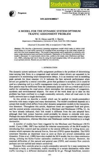
  • 8. 162 M.O. GHALI andM.J. SMITH Fig. 4. Geometry of Network 1. each link rather than the user equilibrium. Total travel delays are reduced by about 20%. Only two iterations were needed for the LMD solution. The UE solution was observed after five iterations. 4.2. zyxwvutsrqponmlkjihgfedcbaZYXWVUTSRQPONMLKJIHGFEDCBA Network 2 This network represents a town in England. It has 250 links and 50 junctions. The results in Fig. 6 show that network performance corresponding to LMD is better than the performance corresponding to UE; total travel delays are reduced by about 3%. Four iterations were needed for the LMD solution. The UE solution was observed after eight iterations. RONETSresults for the network in Allsop (1977) 27000 26000 25ooo B ‘n 24000 23000 ._ 2 3 4 5 Iteration Fig, 5. Performance of Network 1under user equilibrium and local marginal delay assignment.
  • 9. Dynamic system optimum traffic assignment 163 RONETS results for a town in England (250 links, 50 junctions) 555000 , a I I I 550000 530000 525000 zyxwvutsrqponmlkjihgfedcbaZYXWVUTSRQPONMLKJIHGFEDCBA 0 1 2 3 4 5 6 I 8 Iteration Fig. 6. Performance of Network 2 under user equilibrium and local marginal delay assignment. 5. THE OPTIMALITY OF THE SOLUTION OF THE MODEL The ability of the method to deal with many origin-destination and many bottleneck networks in a dynamic context has been demonstrated in the network tests provided. The method, on the other hand, is approximate, and as such it may not produce an optimal solution. The method is approximate due to the following limitations of the local mar- ginal delay, viewed on a route level: 1. Route marginal delays based on the local marginal delay of each link along the route do not necessarily determine the steepest descent direction. 2. Route marginal delays based on the local marginal delay of each link along the route do not necessarily determine a descent direction, at all. We will not address in this article issues relating to uniqueness, convexity/noncon- vexity and differentiability of the model presented here. These have recently been ad- dressed in Ghali and Smith (1993), where it is particularly shown that the dynamic system optimum problem may generally not have a unique solution and may be a nonconvex and nondifferentiable problem. Also in Ghali and Smith (1993) a different marginal delay system, overcoming some of the shortcomings of the marginal delay system of this article, is described. (An algorithm based on this different marginal delay system is presented in Ghali and Smith, 1992.) Next, we explain the limitations of the local marginal delay. zyxwvutsrqponmlkjihgfedcbaZ 5. I. Route marginal delays, based on LMD, do not necessarily determine the steepest descent direction The model considers only the local marginal delay of each link while rerouting each vehicle. In the steady state, rerouting vehicles along the routes which have least link (local) marginal delay determines the least costly pattern of flow (if the total delay function is convex; see Dafermos and Sparrow, 1969). Regrettably, this feature does not carry over to the dynamic state. This is so because route marginal delays, based on adding the local marginal delay of each link along the route, do not be always global, except for some network topologies. To show that route marginal delay may not always determine the steepest descent direction, we consider the network shown in Fig. 7. This is similar to the network consid- ered in Appendix A and shown in Fig. 8. Here it is modified slightly to allow for route
  • 10. 164 M.O. GHALI andM.J. SMITH Fig. 7. Network showing two route choices for commodity 02 = D2. choice between 02 to D2 by adding the route 02-5-6-D2. Traveling time on route 02-5- 6-D2 is assumed to be equal to 6 seconds. Travel times on other links, bottleneck capaci- ties and commodity demands are as in Appendix A. For this example, the optimality of the solution based on link-local marginal delays, and as obtained by our model, will depend on the value of 6. Because we are interested in establishing that route marginal delays do not necessarily determine the steepest descent direction, we will take a value for 6 which shows this clearly. The chosen value of 6 is 125 seconds. This value is greater than the largest value of the marginal delays at bottleneck Bl, which is 120 seconds. This value of 120 seconds corresponds to the case in which all the flow of commodity 2 travels through Bl; in this case the queue dissipates at Bl at time 120 seconds and the total travel delays are 121,500, as in Appendix A. Now consider swapping some of the flow rate from commodity 2 to take the route 02-5-6-D3. Let the swap value be Eveh/sec, out of the total demand 10veh/sec. The total travel delays (networkwide) then become 180 x (E - 10) x (-27,000 + 2000~ - 50~~ + E~)/( -20 + e)* + 7500~ (3) and the gradient of the total travel delays, with respect to E, is 300 x (200,000 - 26,500~ + 1800~’ - 70C3 + E4)/( -20 + E)3 + 7500. (4) For E = 0, the total travel delays are, as before, 121,500 veh/sec, and the gradient is equal to - 1500, which is negative. So the networkwide travel delays can be reduced by swapping some of the flow of commodity 2 from route 02-5-6-D2 to route 02-5-6-D2 (or by moving in the direction of positive values of E, from the bottom to the top route). However, with the value of 6 being 125 seconds and the largest value of the local marginal delays at Bl being 120 seconds, no traffic from commodity 2 will be forced to take route 02-5-6-D3 when routing traffic from commodity 2 according to these marginal delays, because the local marginal delay at Bl ( = 120) is less than 6 ( = 125) on route 02-5-6-D2. Fig. 8. An example network with three commodities and two bottlenecks.
  • 11. Dynamic system optimum traffic assignment 165 In view of this example, the model does not in general determine a system optimum pattern of flow. Nonetheless, in the single-bottleneck-per-route case, our algorithm can be guaranteed to determine the system optimal pattern of flow. This single-bottleneck case is introduced in Smith and Ghali (1990) and corresponds to a network in which each reasonable route connecting each origin-destination pair in the network passes through no more than a single active bottleneck. 5.2. zyxwvutsrqponmlkjihgfedcbaZYXWVUTSRQPONMLKJIHGFEDCBA Route marginal delays, based on LMD, do not necessarily determine a descent direction, at all Here we show that route marginal delays based on link-local marginal delays may not always determine a descent direction, We consider the preceding example again, but here we assume that initially all the flow of commodity 2 is on route 02-5-6-D2. In this case total travel delays from eqn (3) are 75,000, and no queues exist at bottleneck Bl. Because no queues now exist, the marginal delay at Bl is thus equal to zero, which is considerably less than the value of 6. So the route marginal delays along route 02-l-3-D2 (having a zero value) are less than those along route 02-5-6-D2 (having a value of S). In spite of that, moving some of the flow of commodity 2 in the direction from the top route to the bottom route increases the total travel delays, because the gradient in eqn (4) at E = 10 is positive in this direction. Hence, the route marginal delays are not pointing in the direction which reduces the total travel delays. 6. CONCLUSIONS AND FURTHER WORK This article presented a model for approximately solving the dynamic system opti- mum problem; the model is based on the local marginal delay of each link. We have also shown that the local marginal delay has two limitations-namely, that in contrast with the steady state, route marginal delays based on adding up the local marginal delay of each link do not necessarily determine the steepest direction nor do they necessarily determine a descent direction in the dynamic state. Results for two networks were given. These show that there are benefits from routing vehicles according to the local marginal delay, in spite of the aforementioned limitations. Finally, Appendix B described a net- work loading procedure. This may prove useful in other related topics, such as route guidance and equilibrium problems. The work in this article may be extended in a number of ways. For instance, consider the computational issue. The computational effort needed to determine the solution of the model may be reduced by constructing a different version of the algorithm which may be implemented on a parallel machine. Similarly, the network loading procedure computational time may also be reduced by implementing it on a parallel machine. In a different direction, it would be interesting to design a procedure which deter- mines the road prices corresponding to the local marginal delay system presented in this article. The local marginal delay cannot be directly translated into efficient road prices, because the intention of the marginal delay is to influence route choice in this article. For example, consider a single-link-bottleneck network that has a travel demand exceeding the capacity of the bottleneck during the rush hour. Here there is no route choice; however, the local marginal delay for a vehicle arriving at the bottleneck at the beginning of the rush hour can be substantial because it corresponds to the difference between the time the vehicle arrives and the time at which the queue at the bottleneck ceases to exist. But if we were only concerned with route choice to reduce congestion, the road prices should be zero. Thus, this is not equal to the (large) marginal delays at this link bottle- neck. Acknowledgements-The authors would like to express their gratitude for the many valuable comments made by an anonymous referee on an earlier version of this article. The work reported here has been partly funded by the Science and Engineering Research Council of the United Kingdom.
  • 12. 166 M.O. GHALI andM.J. SMITH REFERENCES Addison, J. D., & Heydecker, B. ( 1993). A mathematical model for dynamic traffic assignment. In C. Daganzo (Ed.), zyxwvutsrqponmlkjihgfedcbaZYXWVUTSRQPONMLKJIHGFEDCBA Proceedings of the 12th International Symposium on Transportation and Traffic Theory (pp. 171- 184). New York: Elsevier. Allsop, R. E., & Charlesworth, J. A. (1977). Traffic in a signal-controlled road network: An example of different timings inducing different routings. Traffic Engineering and Control, 18, 262-264. Bellman, R. E. (1958). On a routing problem. Quart. Appl. Math., 26, 87-90. Bernstein, D., Friesz, T. L., Tobin, R. L., & Wie, B-W. (1993). A variational control formulation of the simultaneous route and departure-time choice equilibrium problem. In C. Daganzo (Ed.), Proceedings of the 12th International Symposium on Transportation and Traffic Theory (pp. 107-126). New York: Elsevier. Carey, M. (1986). A constraint qualification for a dynamic traffic assignment model. Transportation Science, 20(l), 55-58. Carey, M. (1987). Optimal time-varying flows on congested networks. Operations Research, 35(l), 58-69. Dafermos, S. C., & Sparrow, F. T. (1969). The traffic assignment problem for a general network. J. Res. Nat. Bureau of Standards-B MathematicalSciences, 73B(2), 91-I 18. Dijkstra, E. W. (1959). A note on two problems in connexion with graphs. Numerische Mathematik, 1, 269- 271. Friesz, T. L., Luque, F. J., Tobin, R. L., & Wie, B. W. (1989). Dynamic network traffic assignment considered as a continuous time optimal problem. Operations Research, 35, 58-69. Ghali, M. O., & Smith, M. J. (1992). Approximation to optimal dynamic traffic assignment of peak period traffic to a congested city network. Paper presented at the 2nd International Capri Seminar on Urban Traffic Networks, Capri, Italy, July 5-8. Ghali, M. O., & Smith, M. J. (1993). Traffic assignment, traffic control and road pricing. In C. Daganzo (Ed.), Proceedings of the 12th International Symposium on Transportation and Traffic Theory (pp. 147- 170). New York: Elsevier. Merchant, D. K., & Nemhauser, Cl. L. (1978a). A model and an algorithm for the dynamic traffic assignment problem. Transportation Science, I2( 3), 183-199. Merchant, D. K., & Nemhauser, G. L. (1978b). Optimality conditions for a dynamic traffic assignment model. Transportation Science, I2( 3), 200-207. Smith, M. J. (1993). A new dynamic traffic model and the existence and calculation of dynamic user equilibria on congested capacity-constrained road networks. Transportation Research, 27B( I). 49-63. Smith, M. J., & Ghali, M. 0. (1990). Dynamic traffic assignment and dynamic traffic control. In M. Koshi (Ed.), Proceedings of the Ilth International Symposium on Transportation and Traffic Theory (pp. 273- 290). New York: Elsevier. APPENDIX A: FLOW CONTROLS IN A MULTI-COMMODITY NETWORK: AN EXAMPLE Consider the network shown in Fig. 8. In this network, three commodities are observed, commodity 1 corresponding to the origin-destination pair Ol-Dl, commodity 2 to 02-D2, and commodity 3 to 03-D3. For simplicity, traveling time on links is taken as zero. Further, the network is assumed to have two bottlenecks; the first is located at the exit of link l-2, denoted as zyxwvutsrqponmlkjihgfedcbaZYXWVUTSRQPONM Bl , and the second at the exit of link 3-4, denoted as B2. Each bottleneck has a capacity of 10veh/sec. The demand from 01 and 02 starts at time t = 0 seconds, at a rate of 10 veh/sec, for a period of 60 seconds. The demand from 03 starts at t = 60 seconds, at a rate of 10 veh/sec, and continues for 5 hours at this rate. Now we consider two cases: ( 1) Traffic from commodity 2 is held back at node 1, perhaps by means of a traffic controller which acts as a flow-control variable in this case; and (2) traffic from commodity 2 merges with traffic from commodity 1 at node 1. In the first case, when traffic of commodity 2 is held back at node I, the traffic from commodity 1 could proceed through the first and second bottlenecks without having to queue at either bottleneck. The total travel delavs in this case are iust aueueina delays of value 36,ooOveh/sec due to holding the traffic from commodity 2 at node 1. Note that traffic-from commodity 3 in this case passes through the second bottleneck without having to queue, because all the traffic from commodity 1 would have arrived at its destination by the time traffic from commodity 3 starts entering the bottleneck. On the other hand, in the second case, when traffic from commodity 2 merges with traffic from commodity I, queues at both bottlenecks Bl and B2 then develop. In this case, precisely half the demand from commodity 1 emerging from the first bottleneck Bl would merge with flow from commodity 3, thus increasing the queueing delay from 36,000 to 121,500 veh/sec, which is a substantial increase in total travel delays. It is clear, therefore, from this example that the total travel time is reduced if the traffic of commodity 2 was held back at or before node 1. However, in the absence of a control mechanism (e.g. a traffic light at node I), it is not possible to hold traffic from commodity 2 merging with the traffic from commodity 1 in entering the bottleneck Bl. APPENDIX B: A METHOD FOR LOADING THE NETWORK In the steady state, loading of the network is straightforward. Given the routes and the route flows, the flow on a link can be calculated by addina all the route flows entering the link. Having found the link flows,the total network delay can then be readily calculated, perhaps utilising a proper delay function for every link. In the dynamic state, the aforementioned nicety does not carry over due to the additional time component.
  • 13. Dynamic system optimum traffic assignment 167 v,w V(t) of slope vg zyxwvutsrqponmlkjihgfedcbaZYXWVUTSRQPONM 11 k t3 Fig. 9. 3-time slice incomplete queue profile. To account for this we describe in this section a method which goes forward in time. We call this a time-slice-by- time-slice loading procedure. The lengths of the time slices in this loading procedure are chosen so that none is greater than the shortest link (uncongested) travel time in the network. The reason for restricting the time slices as such is given next. The lime-slice-by-rime-slice loading procedure As in the main body of this article, we call the profile depicted in Fig. 1, which expresses the relation between the entry and exit flow of a particular link bottleneck the queue profile of the link bottleneck. We will also call a bottleneck queue profile of a bottleneck which is determined up to the end of a certain time slice, which is not the last time slice of the modeling period, a bottleneck incomplete queue profile. Figure 9 shows an incomplete queue profile for some link bottleneck determined up to the third time slice; Fig. 10 shows the same queue profile but with one time slice added; Fig. 1 shows the complete queue profile. In explaining this loading procedure, we will start from a point at which all the link queue profiles are calculated and stored up to the end of a certain time slice. [Storing of the queue profile for some link and some time slice within the planning horizon requires storing the initial queue length at the beginning of the time slice and the inflow rate into the link within the time slice. Knowledge of these two values enables one to calculate v,w V(t) of slope VJ between t2and ts. 4 tz t3 t Fig. IO. 4-time slice incomplete queue profile.
  • 14. 168 M.O. GHALI andM.J. SMITH the queueing delays for any vehicle joining the back of the queue on the link within the time slice. Of course, this is only because we assumed the inflow rate into each link bottleneck as constant; see eqns (5) and (a).] Then it is necessary to complete the queue profile of a certain link beyond that certain time slice to account for the queues in the current time slice and beyond. Following the same argument, it then becomes easy to determine the queue profile of other links within the same current time slice and for subsequent time slices. Some of the vehicles within the current time slice will be newly arising from the origin nodes and others will be continuing to their respective destinations. The effects of these vehicles on the network in regard to the total delay have yet to be considered before exiting the network. For vehicles which have arrived at their destination before the current time slice, their effect on the network is assumed to have been considered already and their total delay calculated, as in the following discussion. Consider some link I connected to a number of upstream links which feed into link I. Denote the set of the upstream links as B(I). The arrival rate at the bottleneck of link I for the current time slice, say s, can be made known from the expression where fk is the size of vehicle k, and pr - j - I means that ( 1) vehicle k is entering link I from some link j in B(I) or an origin situated at the beginning of link I, and (2) vehicle k joins the back of the queue at the end of link I within the current time slice. Having calculated the arrival rate at the bottleneck of link I within the current time slice, it remains to calculate ( 1) the delay encountered on link I by each vehicle k; and (2) the delay further downstream, if vehicle k exits link I in the current time slice and proceeds into a downstream link and joins the back of the queue at the end of the downstream link within the current time slice. If the vehicle does not arrive at the bottleneck of the downstream link within the current time slice, its effect is then taken into consideration in the following time slice. If not, the vehicle would have exited the network at the end of link I. If the vehicle did exit the network, its route delay is added to the total route delay of all the vehicles which have already left the network. The queuing delay encountered on link zyxwvutsrqponmlkjihgfedcbaZYXWVUTSRQPONMLKJIHGFEDCBA I by some vehicle k joining the back of the queue at time tP within the current time slice can be computed from (4; + (4 - w,)t%)/w, (6) where 4: is the queue length at the beginning of the current time slice s and w,is the capacity or the service rate of link zyxwvutsrqponmlkjihgfedcbaZYXWVUTSRQPONMLKJIHGFEDCBA I (assumed constant for all time slices). To calculate the queueing delay further downstream on a do .rstream link, say u, the exit time of each vehicle from the upstream links, including link I, should be first calculated from expressions such as eqn (6) for every upstream link connected to U. This means that the queue profiles, up to the end of the current time slice, of every upstream link connected to link u should have been made known before the queue profile and hence the total delay of the vehicles entering u can be calculated on link u. The loading procedure should be performed for each link and for each time slice, but following some order. In other words, the queue profile of a link within a specified time slice cannot be calculated unless all the links upstream of this link have had their queue profiles calculated up to the current time slice (or the end of the previous time slice if the vehicles emerging from the upstream links cannot reach the back of the queue on this link in the current time slice). A natural order in calculating the link queue profiles for all the links would be to start first from the origin nodes. But for a reason that will become obvious later, we require that none of the time slices discretising the study period into a number of time slices should be greater than the time needed to traverse the shortest link in the network. Starting from the origins, in the first time slice, no vehicles will exit any of the links because we assumed that none of the time slices is larger than the time needed to traverse the shortest link in the network. In this time slice, all the vehicles which can reach the bottleneck on the links downstream of the origin nodes are considered in calculating the first time slice of the link queue profiles. Those vehicles which did not reach the bottleneck are considered as arriving later in a subsequent time slice, and their effects on the link queue profile has yet to be considered. In the second time slice, all the vehicles which could exit the links on their routes in the first time slice and could reach the downstream bottlenecks on the downstream links of their routes in this second time slice are used to calculate the second time-slice part of the link queue profiles on the down- stream links. In addition, any vehicles which did not reach the bottleneck of the links downstream of the origins in the first time slice are included in the calculation of the second time slice of the link profiles if they do reach the bottleneck now. Any newly arising flow from the origins in this second time slice is considered in calculating the second time-slice part of the link queue profiles of the links downstream of the origin nodes if it reaches the bottlenecks in this second slice. After the second slice, the foregoing procedure is repeated until finally, by the end of the last time slice of the planning horizon, all the links will have had their link queue profiles calculated, all the vehicles will have arrived at their destinations and the total delay will have been noted. Next we illustrate why we require that none of the time slices discretising the study period into a number of time slices should be greater than the time needed to reverse the shortest link in the network. Consider the network shown in Fig. 1I. In this network we assume that all the turning movements are permitted and all the routes have positive flows. Suppose we are calculating the nth time-slice part of the queue urofile of link I. If the nth time slice is too long, the nth time-slice of the queue profile of link I is affected by the iight-turn flow emerging from link 3, the nth t’lmeslice of the queue profile of link 3 is affected by the right-turn flow emerging from link 2 and the nth time slice of the queue profile of link 2 is affected by the right-turn flow emerging from link 1, then the nth time slice of the queue profile of link 1 cannot be calculated. This is like a deadlock in computer terminology, wherein each process is waiting for the other to finish. However, with a restriction on the length of each time slice corresponding to the time to traverse the shortest link, this deadlock
  • 15. Dynamic system optimum traffic assignment 169 Fig. 11.Network with six origin-destination pairs. does not arise. This is mainly because the nth time-slice part of the queue profile of link I is affected by the right-turn flow emerging from link 3 in a previous time slice, and so on for links 3 and 2, which are affected by the flow of a previous of a previous time slice. To put it differently, for the too long nth time slice, the chain- ( 1,nth time slice), (3, nth time slice), (2, nth time slice), ( 1, nth time slice)-is closed if it is read from left to right to indicate that a (link, time slice) combination is dependent on its adjacent to the right. In this case, both ends of the chain are interdependent. In contrast, for a sufficiently short time slice, the aforementioned chain becomes open because both end combinations, although they have a common link (I), would now have different time slices. FIFO sutisfied. So far we have discussed how the queue profiles are calculated. We still need to mention how FIFO is satisfied in the aforementioned loading procedure. Consider now any two vehicles a and b, joining the back of the queue on some link i within a time slice s. Suppose that the time vehicle u joins the back of the queue on link j is earlier than the time vehicle b does. Let the time when vehicle u joins be t: and that of vehicle b be tz. Also, let the time when vehicle a departs from the queue be tf, and similarly let that of vehicle b to t$. Obviously, tz < t%.It remains to show that tl c tf. If this relation is satisfied, then we have FIFO. From eqns (5) and (a), we have for vehicle u and for vehicle b, tf = {q’o + (v; - w,)t:}/w, + t:, 1; = {q”o+ (v; - w,)tZ}/w, + 18. The terms t: and 18can be written in terms of ti and t$ respectively, to get t: = {w,ti - qi}/vf, and tj = {wti - qi}/vf. Because tz < t$,this implies {WY::- q;}/v; < (w,tll - q;}/v;. After dropping and subtracting common terms, we get hence FIFO. The preceding FIFO argument considers only two vehicles within a common time slice. For vehicles joining the queues in different time slices, a similar construction can be made to show that even then FIFO is satisfied. We omit this here. APPENDIX C: AN ALGORITHM BASED ON THE LOCAL MARGINAL DELAY Notations p = The number of vehicles constituting the total demand from all origins. k = A vehicle number or identification. L = Number of links in network. r, = Uncongested travel time on link 1. q: = Queue length in front of vehicle k on link I when joining the back of queue, if any. w, = Capacity of the bottleneck of link 1.
  • 16. 170 M. 0. GHALI and M. J. SMITH i = Iteration counter. p: = Route of vehicle kin iteration zyxwvutsrqponmlkjihgfedcbaZYXWVUTSRQPONMLKJIHG i. fk = Size of vehicle k (assumed 1 in this article). C’ = Total travel costs (or delays) in iteration i, summed up over all vehicles and links. This is the expression: k=g ,=I. 2 ,2fk( f/+d/w,) Steps 1. i = 0. 2. Calculate and store the route of each vehicle which minimises the route delays of the vehicle, based on uncongested link travel time. Let the route of vehicle k be pi. 3. Calculate total travel delays, C’(using the loading procedure described in Appendix B). 4.Letk=l,i=i+ landC’=C’-‘. a. Remove vehicle k from each link on route pi-‘. This entails updating the inflow rates into each link and each link bottleneck on route pi-‘. Only those inflow rates corresponding to the time slices during which vehicle k enters are updated. b. Determine new route p: on the basis of the values of m obtained from profiles similar to Fig. 1 for each link. c. Assign vehicle zyxwvutsrqponmlkjihgfedcbaZYXWVUTSRQPONMLKJIHGFEDCBA k to its new route by updating the inflow rates of the corresponding time slices within which vehicle k enters the links and the link bottlenecks on route p:. d. Calculate total travel delays TC (using the loading procedure described in Appendix B). If TC < C’, then the new route of vehicle k is favourable and the old route piv’ is replaced by pi and C’ is made equal to TC. Otherwise, C’ and p: are left unchanged. e. If k = p, then go to step 5. Otherwise, increment k by 1 and return to step 4a. 5. If C’ cr C’-‘, return to step 4. Otherwise, the algorithm is terminated. APPENDIX D: AN ALGORITHM BASED ON LINK TRAVEL DELAYS The notations are as in Appendix C. Steps 1. i = 0. 2. Let k = 1, i = i + 1. a. If i is greater than 1, then remove vehicle k from each link on route p);‘. This entails updating the inflow rates into each link and each link bottleneck on route pk-‘. Only those inflow rates corresponding to the time slices during which vehicle k enters are updated. b. Determine new route pi on the basis of the link delay of each link. c. Assign vehicle k to its new route by updating the inflow rates of the corresponding time slices within which vehicle k enters the links and the link bottlenecks on route pi. d. If k = p, then go to step 3. Otherwise, increment k by 1 and return to step 2a. 3. If new routes were allocated, return to step 2. Otherwise, the algorithm is terminated.