Downloaded 49 times
![sample point. Typical attributes included envelope,
bandwidth, impedance, amplitude variation with offset
(AVO) slope and intercept, dip magnitude, and coher-
ence. These attributes were projected onto a 2D latent
space and their results plotted against a 2D color table.
Gao (2007) applies a 1D SOM to gray-level co-occur-
rence matrix (GLCM) texture attributes to map seismic
facies offshore Angola. Overdefining the clusters with
256 prototype vectors, he then uses 3D visualization
and his knowledge of the depositional environment
to map the “natural” clusters. These natural clusters
were then calibrated using well control, giving rise to
what is called a posteriori supervision. Roy et al.
(2013) build on these concepts and develop an SOM
classification workflow of multiple seismic attributes
computed over a deepwater depositional system. They
calibrate the clusters a posteriori using classical princi-
ples of seismic stratigraphy on a subset of vertical slices
through the seismic amplitude. A simple but very impor-
tant innovation was to project the clusters onto a 2D
nonlinear Sammon space (Sammon, 1969). This projec-
tion was then colored using a gradational 2D color scale
like that of Matos et al. (2009), thus facilitating the in-
terpretation. Roy et al. (2013) introduce a Euclidean dis-
tance measure to correlate predefined unsupervised
clusters to average data vectors about interpreter de-
fined well-log facies.
Generative topographic mapping (GTM) is a more re-
cent unsupervised classification innovation, providing a
probabilistic representation of the data vectors in the
latent space (Bishop et al., 1998). There has been very
little work on the application of the GTM technique to
seismic data and exploration problems. Wallet et al.
(2009) are probably the first to apply the GTM tech-
nique to seismic data, using a suite of phantom horizon
slices through a seismic amplitude volume generating a
waveform classification. Although generating excellent
images, Roy (2013) and Roy et al. (2014) find the intro-
duction of well control to SOM classification to be
somewhat limited, and instead apply GTM to a Mississip-
pian tripolitic chert reservoir in midcontinent USA and a
carbonate wash play in the Sierra Madre Oriental of
Mexico. They find that GTM provides not only the most
likely cluster associated with a given voxel, but also the
probability that voxel belongs each of clusters, providing
a measure of confidence or risk in the prediction.
The k-means, SOM, and GTM are all unsupervised
learning techniques, where the clustering is driven only
by the choice of input attributes and the number of de-
sired clusters. If we wish to teach the computer to
mimic the facies identification previously chosen by
a skilled interpreter, or link seismic facies to electrof-
acies interpreted using wireline logs, we need to intro-
duce “supervision” or external control to the clustering
algorithm. The most popular means of supervised learn-
ing classification are based on artificial neural networks
(ANNs). Meldahl et al. (1999) use seismic energy and
coherence attributes coupled with interpreter control
(picked seed points) to train a neural network to iden-
tify hydrocarbon chimneys. West et al. (2002) use a sim-
ilar workflow, in which the objective is seismic facies
analysis of a channel system and the input attributes
are textures. Corradi et al. (2009) use GLCM textures
and ANN, with controls based on wells and skilled in-
terpretation of some key 2D vertical slices to map sand,
evaporate, and sealing versus nonsealing shale facies
offshore of west Africa.
The support vector machine (SVM, where the word
“machine” is due to Turing’s [1950] mechanical decryp-
tion machine) is a more recent introduction (e.g.,
Kuzma and Rector, 2004, 2005, 2007; Li and Castagna,
2004; Zhao et al., 2005; Al-Anazi and Gates, 2010). Origi-
nating from maximum margin classifiers, SVMs have
gained great popularity for solving pattern classification
and regression problems since the concept of a “soft
margin” was first introduced by Cortes and Vapnik
(1995). SVMs map the N-dimensional input data into
a higher-dimensional latent (often called feature) space,
where clusters can be linearly separated by hyper-
planes. Detailed descriptions of SVMs can be found
in Cortes and Vapnik (1995), Cristianini and Shawe-
Taylor (2000), and Schölkopf and Smola (2002). Li
and Castagna (2004) use SVM to discriminate alterna-
tive AVO responses, whereas Zhao et al. (2014) and
Zhang et al. (2015) use a variation of SVM using miner-
alogy logs and seismic attributes to predict lithology
and brittleness in a shale resource play.
We begin our paper by providing a summary of the
more common clustering techniques used in seismic fa-
cies classification, emphasizing their similarities and
differences. We start from the unsupervised learning
k-means algorithm, progress through projections onto
principal component hyperplanes, and end with projec-
tions onto SOM and GTM manifolds, which are topo-
logical spaces that resemble Euclidean space near
each point. Next, we provide a summary of supervised
learning techniques including ANNs and SVMs. Given
these definitions, we apply each of these methods to
identify seismic facies in the same data volume acquired
in the Canterbury Basin of New Zealand. We conclude
with a discussion on the advantages and limitations of
each method and areas for future algorithm develop-
ment and workflow refinement. At the very end, we pro-
vide an appendix containing some of the mathematical
details to better quantify how each algorithm works.
Review of unsupervised learning classification
techniques
Crossplotting
Crossplotting one or more attributes against each
other is an interactive, and perhaps the most common,
clustering technique. In its simplest implementation,
one computes and then displays a 2D histogram of
two attributes. In most software packages, the inter-
preter then identifies a cluster of interest and draws
a polygon around it. Although several software pack-
ages allow crossplotting of up to three attributes, cross-
plotting more than three attributes quickly becomes
Interpretation / November 2015 SAE31
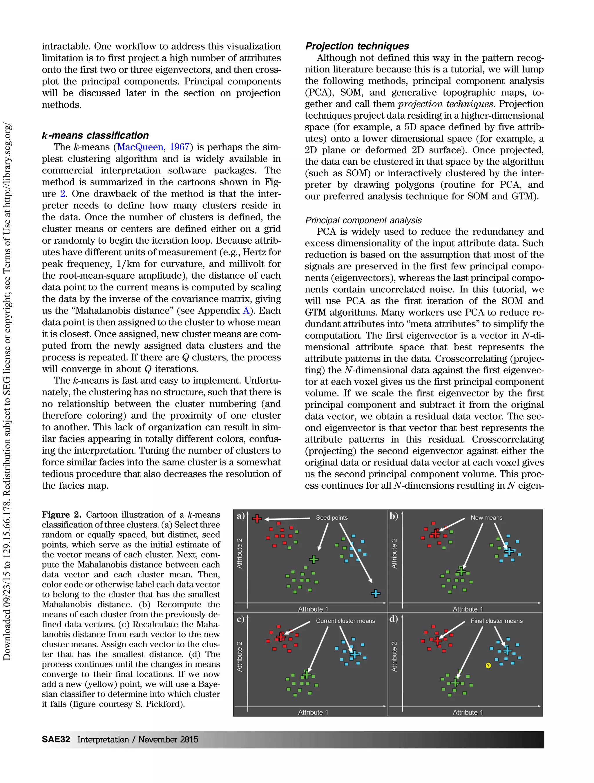
Downloaded09/23/15to129.15.66.178.RedistributionsubjecttoSEGlicenseorcopyright;seeTermsofUseathttp://library.seg.org/](https://image.slidesharecdn.com/vjayaraminterpretation1-151109142231-lva1-app6892/75/A-comparison-of-classification-techniques-for-seismic-facies-recognition-3-2048.jpg)
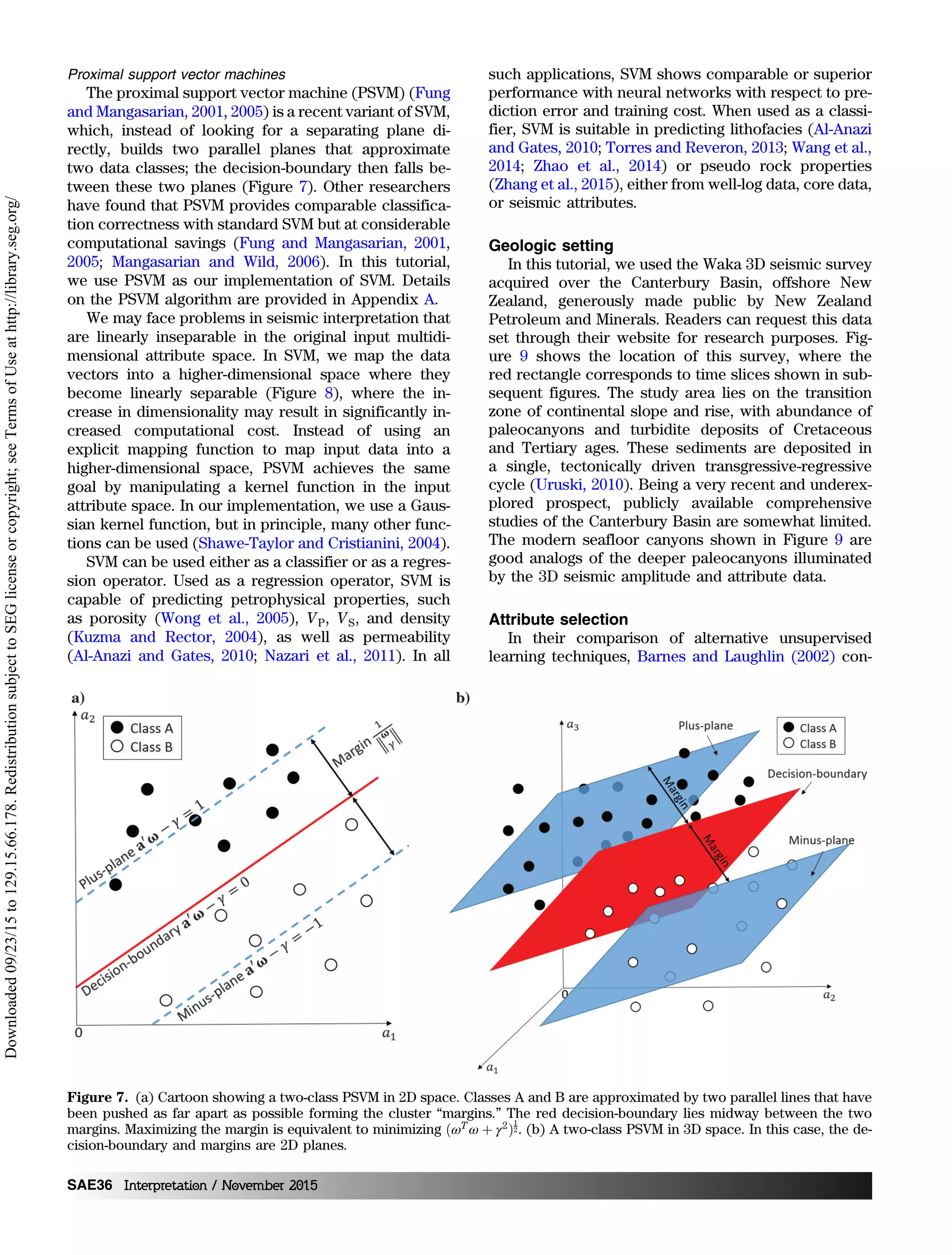
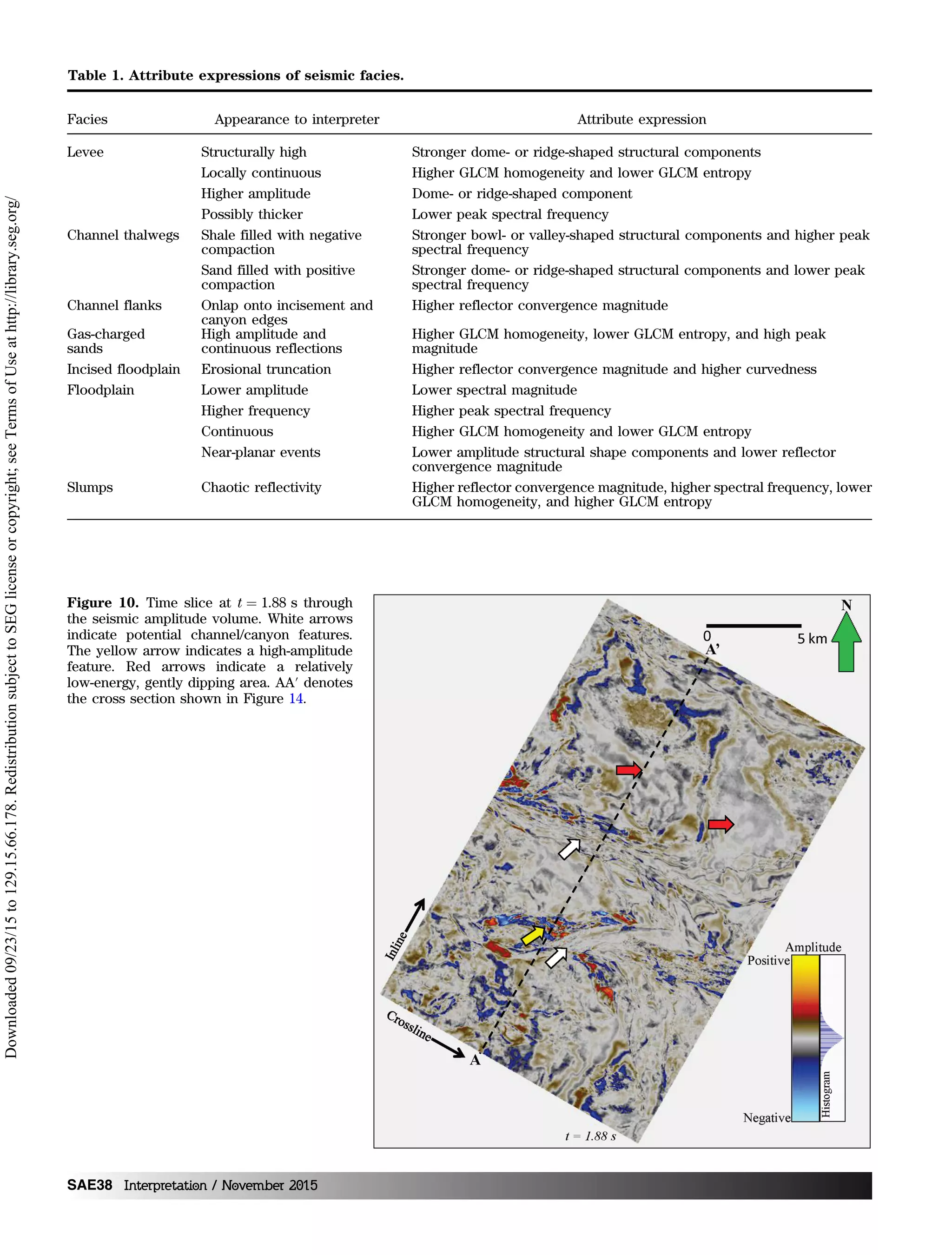
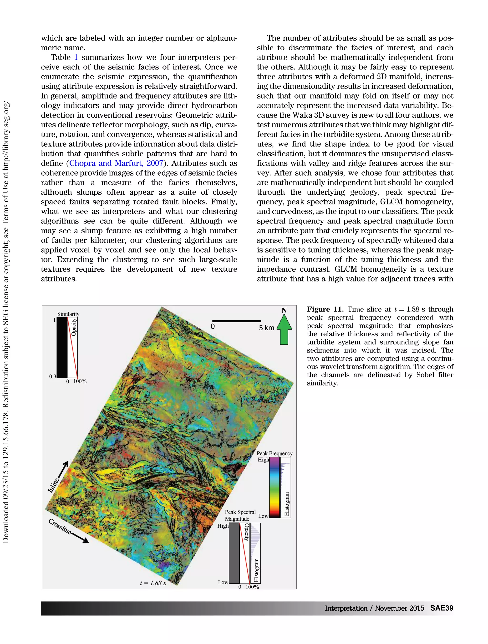
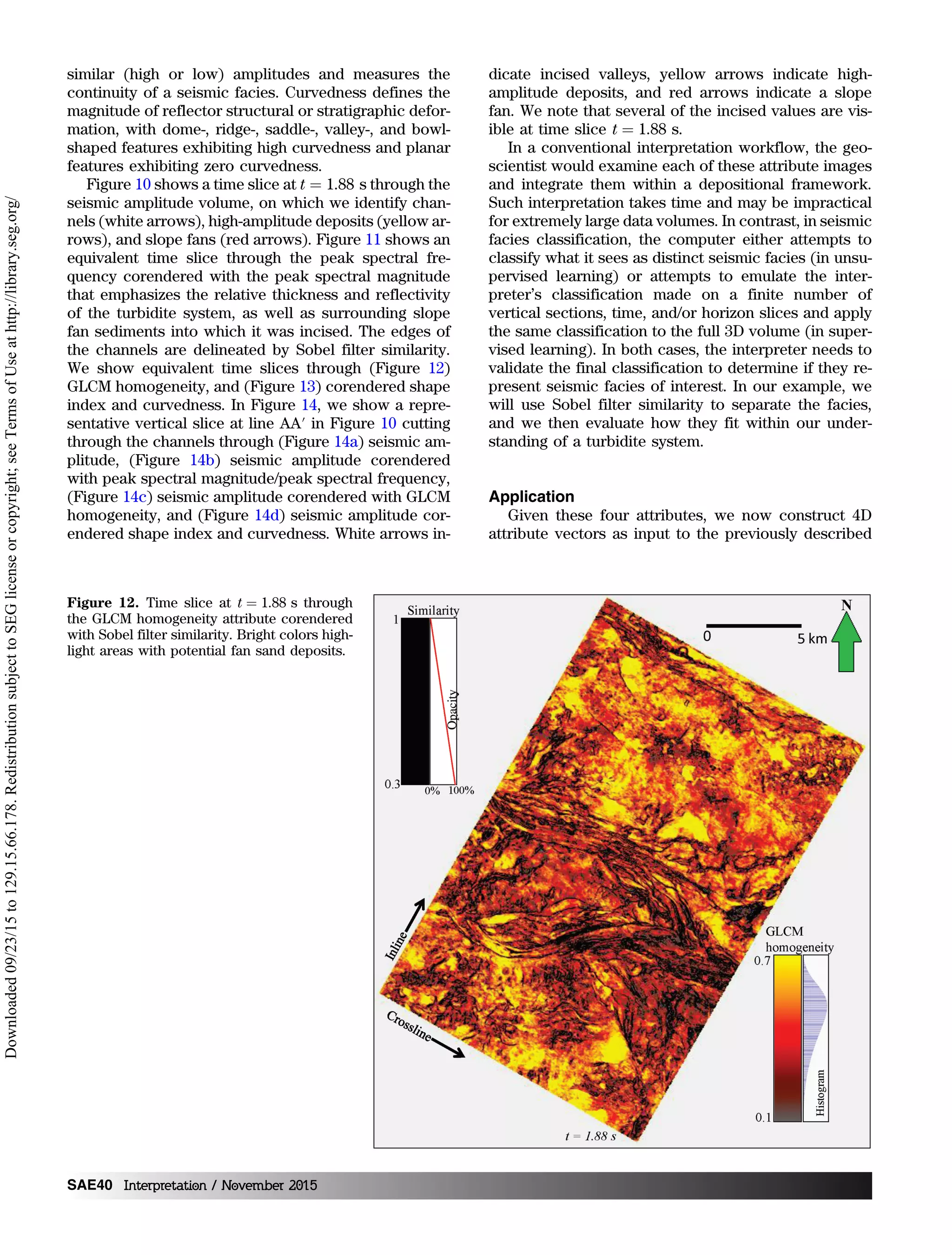
![clude that the appropriate choice of attributes was the
most critical component of computer-assisted seismic
facies identification. Although interpreters are skilled
at identifying facies, such recognition is often subcon-
scious and hard to define (see Eagleman’s [2012] dis-
cussion on differentiating male from female chicks
and identifying military aircraft from silhouettes). In su-
pervised learning, the software does some of the work
during the training process, although we must always
be wary of false correlations, if we provide too many
attributes (Kalkomey, 1997). For the prediction of con-
tinuous data, such as porosity, Russell (1997) suggests
that one begin with exploratory data analysis, where
one crosscorrelates a candidate attribute with the de-
sired property at the well. Such crosscorrelation does
not work well when trying to identify seismic facies,
Figure 9. A map showing the location of the
3D seismic survey acquired over the Canter-
bury Basin, offshore New Zealand. The black
rectangle denotes the limits of the Waka 3D
survey, whereas the smaller red rectangle de-
notes the part of the survey shown in sub-
sequent figures. The colors represent the
relative depth of the current seafloor, warm
being shallower, and cold being deeper. Cur-
rent seafloor canyons are delineated in this
map, which are good analogs for the paleocan-
yons in Cretaceous and Tertiary ages (modi-
fied from Mitchell and Neil, 2012).
Figure 8. Cartoon showing how one SVM can map two linearly inseparable problem into a higher-dimensional space, in which
they can be separated. (a) Circular classes A and B in a 2D space cannot be separated by a linear decision-boundary (line). (b) Map-
ping the same data into a higher 3D feature space using the given projection. This transformation allows the two classes to be
separated by the green plane.
Interpretation / November 2015 SAE37
Downloaded09/23/15to129.15.66.178.RedistributionsubjecttoSEGlicenseorcopyright;seeTermsofUseathttp://library.seg.org/](https://image.slidesharecdn.com/vjayaraminterpretation1-151109142231-lva1-app6892/75/A-comparison-of-classification-techniques-for-seismic-facies-recognition-9-2048.jpg)
![3) Update the winner prototype vector and its neigh-
bors. The updating rule for the weight of the kth
prototype vector inside and outside the neighbor-
hood radius σðtÞ is given by
mkðtþ1Þ
¼
mkðtÞþαðtÞhbkðtÞ½aj −mkðtÞŠ; ifkrk −rbk≤σðtÞ;
mkðtÞ; ifkrk −rbkσðtÞ;
(A-6)
where the neighborhood radius defined as σðtÞ is
predefined for a problem and decreases with each
iteration t. Here, rb and rk are the position vectors
of the winner prototype vector mb and the kth proto-
type vector mb, respectively. We also define the
neighborhood function hbkðtÞ, the exponential learn-
ing function αðtÞ, and the length of training T. The
hbkðtÞ and αðtÞ decrease with each iteration in the
learning process and are defined as
hbkðtÞ ¼ e−ðkrb−rkk2∕2σ2ðtÞ
; (A-7)
and
αðtÞ ¼ α0
0.005
α0
t∕T
. (A-8)
4) Iterate through each learning step (steps [1–3]) until
the convergence criterion (which depends on the
predefined lowest neighborhood radius and the min-
imum distance between the prototype vectors in the
latent space) is reached.
5) Project the prototype vectors onto the first two prin-
cipal components and color code using a 2D color
bar (Matos et al., 2009).
Generative topological mapping
In GTM, the grid points of our 2D deformed manifold
in N-dimensional attribute space define the centers, mk,
of Gaussian distributions of variance σ2 ¼ β−1. These
centers mk are in turn projected onto a 2D latent space,
defined by a grid of nodes uk and nonlinear basis func-
tions Φ:
mk ¼
XM
m¼1
WkmΦmðukÞ; (A-9)
where W is a K × M matrix of unknown weights,
ΦmðukÞ is a set of M nonlinear basis functions, mk
are vectors defining the deformed manifold in the N-di-
mensional data space, and k ¼ 1;2; : : : ; K is the number
of grid points arranged on a lower L-dimensional latent
space (in our case, L ¼ 2). A noise model (the probabil-
ity of the existence of a particular data vector aj given
weights W and inverse variance β) is introduced for
each measured data vector. The probability density
function p is represented by a suite of K radially sym-
metric N-dimensional Gaussian functions centered
about mk with variance of 1∕β:
pðajjW; βÞ ¼
XK
k¼1
1
K
β
2π
N
2
e−β
2kmk−ajk2
. (A-10)
The prior probabilities of each of these components are
assumed to be equal with a value of 1∕K, for all data
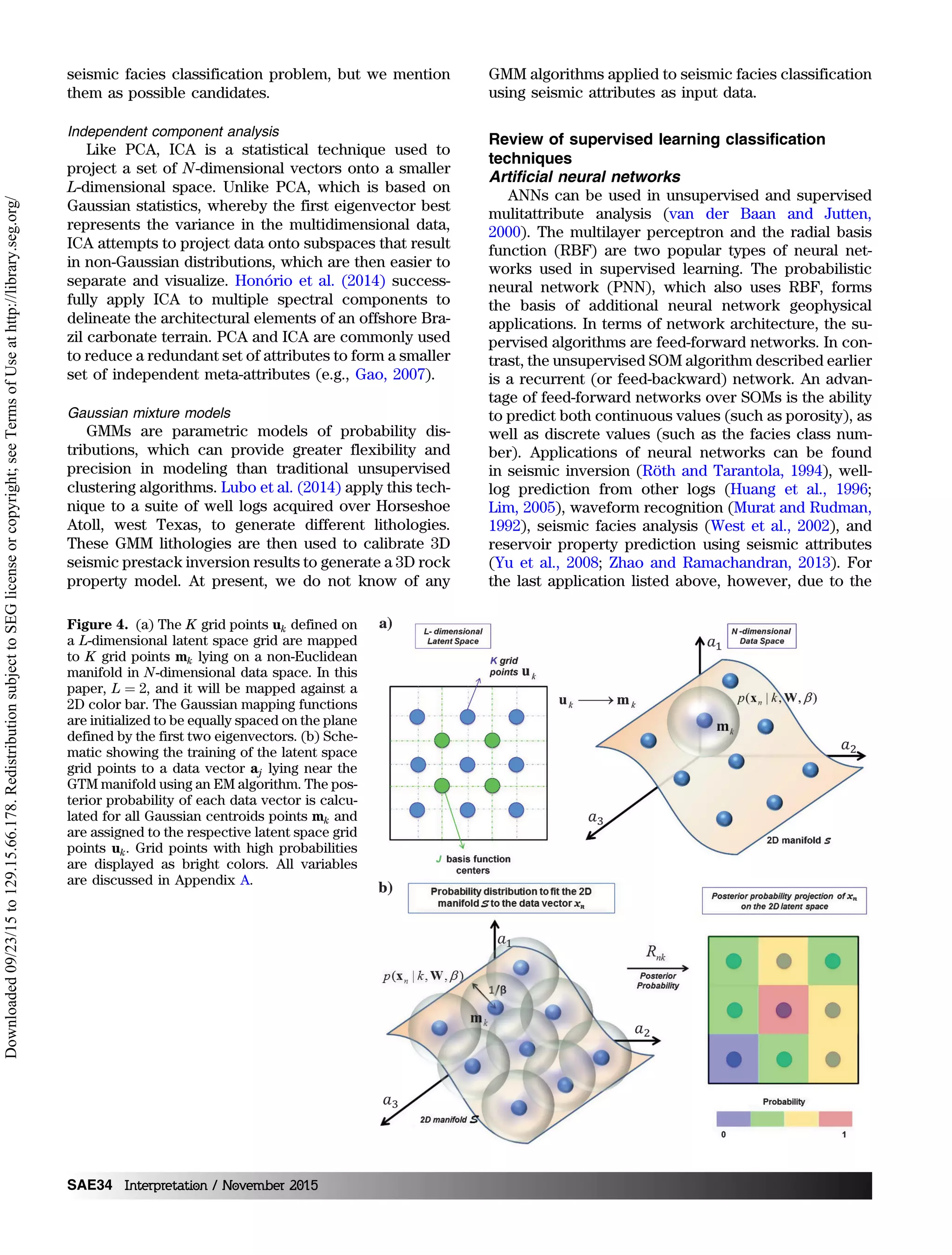
vectors aj. Figure 4 illustrates the GTM mapping from
an L ¼ 2D latent space to the 3D data space.
The probability density model (GTM model) is fit to
the data aj to find the parameters W and β using a maxi-
mum likelihood estimation. One popular technique
used in parameter estimations is the EM algorithm. Us-
ing Bayes’ theorem and the current values of the GTM
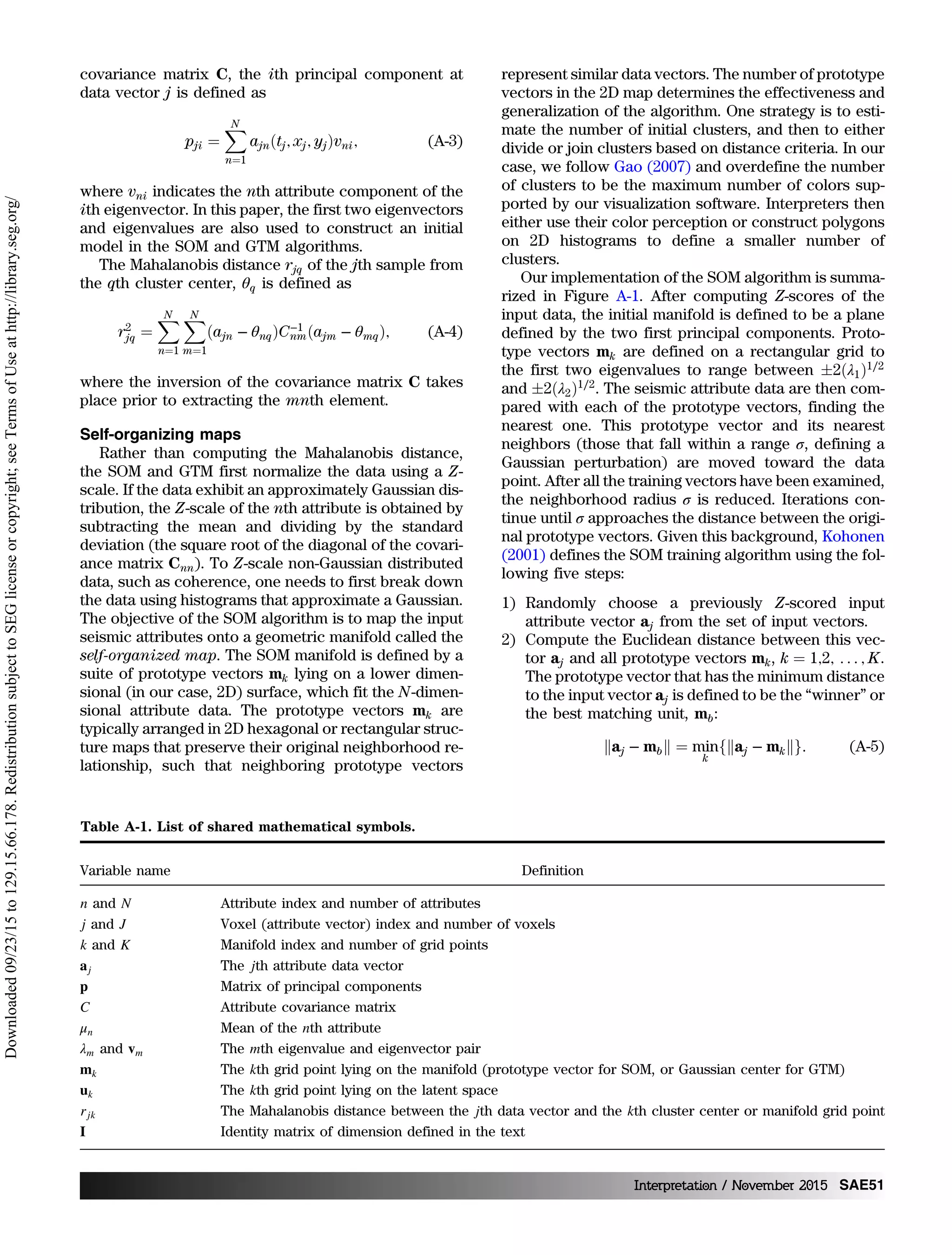
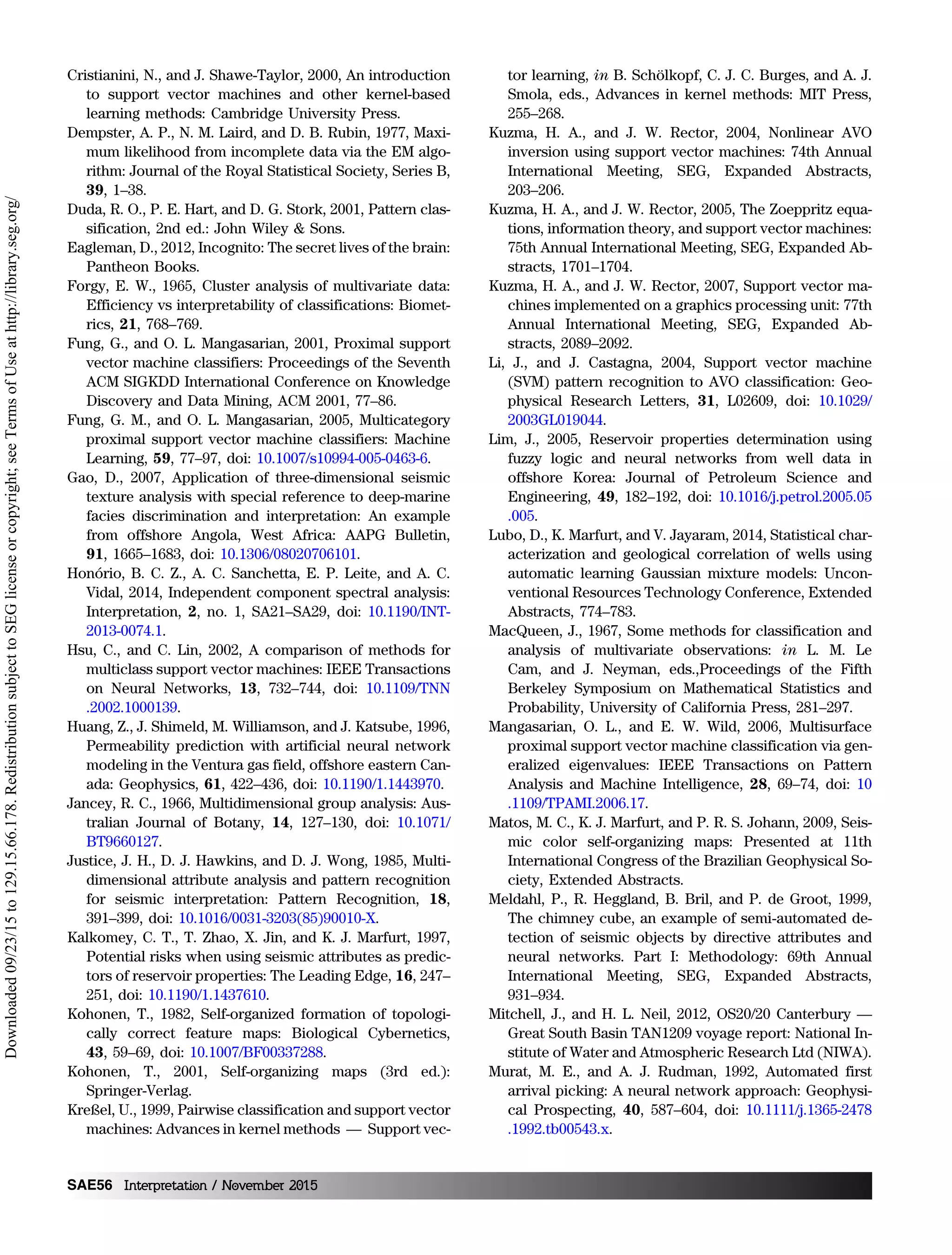
Figure A-1. The SOM workflow.
SAE52 Interpretation / November 2015
Downloaded09/23/15to129.15.66.178.RedistributionsubjecttoSEGlicenseorcopyright;seeTermsofUseathttp://library.seg.org/](https://image.slidesharecdn.com/vjayaraminterpretation1-151109142231-lva1-app6892/75/A-comparison-of-classification-techniques-for-seismic-facies-recognition-24-2048.jpg)

The document reviews several seismic facies classification algorithms applied to 3D seismic data from the Canterbury Basin in New Zealand, including k-means, self-organizing maps, and support vector machines. It highlights the importance of selecting appropriate input attributes and describes how supervised learning techniques can enhance accuracy in identifying seismic facies, while unsupervised methods may reveal overlooked features. The paper concludes by discussing the advantages and limitations of each method and potential future developments in seismic data interpretation.