This document discusses data structures for geographic and cartographic data. It notes that current data structures are characterized by: 1) being designed for input rather than use in programs, 2) storing different feature types in separate uncoordinated files, and 3) lacking information on neighboring entities. The concept of a "neighborhood function" is introduced to indicate an entity's relative location, which is important for analysis. Ongoing research includes the GEOGRAF and GDS systems, which involve manipulating data between input and use to address issues of flexibility, comparability, and topology.

1. * Semiannual Journal of the American Congresson Surveyingand Mapping
430 Woodward Building, 733 15th Street, N.W., Washington, D.C. 20005
Cartographic Data Structures
ABSTRACT. Efficient and flexible data structures are important to the development of
computer mapping. Most current data banks are characterized by 1) structures which
are convenient at the input stage rather than at the stages of use within computer
programs, 2) separate and uncoordinated files for different types of geographic fea-
tures, and 3) a lack of information about neighboring entities. The term "neighbor-
hood function" may be used to indicate the relative location of a geographic entity
and is a concept which is involved in all three of these characteristics. Ongoing re-
search on data structures had led to work on the GEOGRAF system for encoding
planar data and the GDS ("Geographic Data Structure") for encoding three-dimen-
sional surfaces. Both involve data manipulation between the digitizing stage and the
actual use of the data within computer mapping programs.
INTRODUCTION
A series of ongoing research projects
are concerned with efficient and flexible
data structures for geographic and carto-
graphic analysis. The three main points
of concern in the research can be sum-
marized as follows:
1) In most cartographic data banks, the
arrangement of the data is guided by the
input stage. In other words, little ma-
nipulation of the data is performed after
the data have been input into the system
from maps.
2) Cartographers and computer scien-
tists have made few attempts to combine
different types of cartographic information,
for example, height with other cartographic
features. Therefore, the different types of
cartographic entities are stored in different
files and it is usually extremely time-con-
suming to combine them.
3) The data structure is usually very
simple and lacks one facet in particular
which is essential for much geographic and
cartographic analysis-an indication of the
relative location of a geographic entity,
i.e., the position of a geographic entity with
respect to its neighboring entities.
These three points may be abbreviated
with the terms flexibility, comparability,
and topology. This paper will characterize
types of existing geographic and carto-
graphic data systems for planar and three-
dimensional surfaces, especially with re-
spect to these three points. The paper will
also describe attempts which have been
made by the authors to produce data sys-
tems which eliminate some of the problems
of existing ones. The term "neighborhood
function" will playa major role throughout
the paper and will therefore be explained in
more detail in the following section.
NEIGHBORHOOD FUNCTION
When asked for the location of a city, we
will· give the location with respect to a
river, a seacoast, a pass, a neighboring
larger city, or other feature. Rarely will
Thomas K. Peucker is associate professor, hi' .
Simon Fraser University, Burnaby, Canada. we use t e geograp llC coordmates of longi-
Nicholas Chrisman is senior programmer, Lab- tude or latitude, nor will we use map co-
oratory for Compu~erGraphics and Spatial Anal- ordinates. Weare taught in elementary
ysis, Harvard University, Cambridge,Massachu- geography that the geographic coordinates
setts. The research for this paper has been will tell us little about either the large-scale
supported by ONR contract NOOOl4-73-C-OI09
and the Laboratory for Computer Graphics and (site) or small-scale (situation) char-
Spatial Analysis, Harvard University. acteristics of a place. Similarly, if I de-
The American Cartographer, Vol. 2, No.1, 1975, pp. 55-69

2. scribe n'y position on a piece of terrain, I
will not use my map to determine my lo-
cation within the UTM-grid; rather I will
look for nearby relief features (peaks,
rivers, slopes, roads) as orientation char-
acteristics,
In contrast, when a geographic data bank
of any kind is created, it utilizes some kind
of absolute coordinate system. Usually
neither the geographic evaluation at the
time of digiti7.in~ nor the mapping system
used with the data allow the inclusion of
such cartographic features as streets, rivers,
and roads which would give us an indica-
tion of relative location.
While the human user can be aided in
his orientation on a map through overlays
or man comparison. the computer has dif-
ficultv in determininl! relative location. If
the relative location in terms of the closest
points for each of, say, 5,000 points is to
be calculated. the program literally has to
compute every point's distance to every
other point. Indeed, some widely-used
prOl!rams do this computation several times
within one program run.
Some indication of the relative location
of a geographic feature can be very useful:
This neighborhood relationship will be re-
ferred to as a "neighborhood function."
It can be expressed in different ways: as
an explicit or implicit function, or as a dis-
crete function in the form of a table.
The explicit function can be a polynomial
or trigonometric equation set for a discrete
grid of surface patches which give the form
of the surface at each point within the
patch. Typical for this approach is the
work of Junkins, et al. (1973). Two-
dimensional spline functions also fall into
this category (Holroyd and Bhattacharyya.
1970). A much more frequent way of de-
fining a neighborhood is by the explicit
function in the form of a sort routine which
finds the closest neighbors. This is done
in various interpolation algorithms to pro-
duce a regular grid of points (Shepard,
1968; Heiskanen and Moritz, 1967). The
computations increase close to the square
of the increase in the number of points,
since the search has to be repeated for
every point and all points, or at least a
large number of them, must be processed
each time.
This search procedure also applies in
the case of planar surfaces where neigh-
boring polygons must be found. For ex-
ample, when contiguity constraints are im-
posed in problems of factorial ecology and
other regional correlations, all polygon
points must be searched to find those which
are in common for a pair of polygons.
Again, the problem increases in complexity
according to the square of the number of
the items being searched.
The implicit function expressing neigh-
borhood relationships is usually a function
that describes the coding structure of the
geographic entities. One very good case
is described in Rosenfeld (1969) for dif-
ferent types of neighborhood relationships
within a regular grid in which the point
Pi; has the four neighbors (i + 1, j), (i.i +
I), (i-I, j), (i. j-I) and it has the eight
neighbors (i + I, j), (i + I, j + I), (1. j + 1),
(i-I. j + I), (i - I, j), (i - 1, j - I), (i, j -
I), (i + 1, j - 1) .
Neighborhood relationships in the form
of tables are very rarely used. This type
records the neighborhood function by
"pointers" indicating neighboring geo-
graphic entities. For example, a structure
which is built on the basis of Thiessen
Polygons could have such a structure by
simply having the labels of the neighboring
points accompany the record of each point.
The most widely-known structure of this
type is the DIME file of the U.S. Census
which encodes line segments, the names of
the polygons to the left and right of each
line segment, and the names of the two
nodes at either end. The neighborhood
relationships used in the DIME develop-
ment are derived from the discipline of
topology (Cooke and Maxfield, 1967) ..if.
Neighborhood relationships will be dis-
cussed in greater detail in the analysis of
various existing data structures. Two
types of geographic data bases win be dis-
cussed: those defining planar surfaces and
those defining three-dimensional surfaces.
For both types, a summary of their his-
torical development will be presented, and
it will be shown that, although presently

3. at different stages of development, these
two types can be treated as special cases
of one topological data structure.
DATA STRUCTURES FOR
PLANAR SURFACES
Types of Structures
The types of geographic entitles on
planar surfaces are points, lines, and area-
enclosing lines or polygons. The latter are
perhaps the most frequently encoded fea-
ture in geographic data systems.
The 'simplestdata base system for planar
surfaces is that of encoding entity by entity
with little or no regard for entity overlaps
or adjacencies (Fig. 1). In other words,
every polygon in a polygon system is en-
coded and stored without any regard for
contiguous polygons, and lines are encoded
without regard for the fact that they may
intersect or merge with other lines. The
results of such an encoding are "sliver
lines" (duplication of lines in slightly dif-
ferent positions). These sliver lines are
confusing and unaesthetic and, hence, it is
virtually impossibleto do anything directly
with such a data base except an extremely
coarse graphic image.
To go beyond the use of such data for
the production of coarse images, editing
must be performed. This alternative has
been attempted in several cases, one being
the MAP-MODEL system (Arms, 1970).
The editing in this system is guided by the
assumption that every segment has to be
represented twice except for segments on
the outer boundary. For each segment,
the editing program sorts through all re-
maining segments to find its complement
(the identical line of the neighboring poly-
gon) . Those segments for which it has
not found a complement are tagged to in-
dicatepotential errors to the user.
To overcome some of the limitations of
independently encoded entities, systems
have been developed based on a common
location dictionary. This dictionary con-
tains the coordinates of every boundary
point on the map. Polygon boundary lists
are then compiled which consist of the
labels (location numbers) of these bound-
ary points (Fig. 2). Line information can
LOCATION LIST
POLYGON 1 x~' Y',l
X~2 Y',2
POLYGON 2 X~,l Y2,'
1,", x2,2 Y2,2
X2,m Y2,m
Fig. 1. The simplest encodingis areal en-
tity by areal entity. In this system, most
points are recorded twice and some (e.g.,
PI,.; PI,ll; Pa,T) three times. A point does
not necessarilyhave identical coordinatesin
all,recordings.
be handled in the same way. Programs
based on this structure include CAL-
FORM from the Laboratory of Computer
Graphics and Spatial Analysis. Other
programs have subroutines to convert this
point dictionary structure to the simple
entity-by-entity line list described above.
The data can then be used in programs
such as SYMAP (Laboratory for Com-
puter Graphics and Spatial Analysis)
wh~ch are. compatible with the entity-by
entIty structure. Programs have also been
developed to simplify data input through
automated polygon identification (Douglas,
1973).

4. POINT DICTIONARY
POINT
1 x Y
2 x Y
3 x y
POLYGON
3 1,25, 24,23.22,21,43,
44,45,46,47, 48. 30.
29. 28. 27, 26, 1
5 44,43,42,41.40.39,
38.37, 36,35, 44
Fig. 2. In the second type of polygon sys-
tem, the individual points are encoded only
once and are stored in the Point Dictionary.
For every polygon, a Polygon Boundary List
is then established.
The point dictionary data base has the
advantage that sliver lines do not occur.
However, the problem of neighborhood
relationships is not handled any better than
with the entity-by-entity approach. The
search for common lines is no longer ac-
cording to the coordinates of points but by
their labels; this brings us closer to a
solution only by a little less computer time.
It also creates difficulties. A point diction-
ary can and will be accessed in an arbitrary
order, since there are no restrictions re-
garding point placement. The standard
response to this problem is to make the
dictionary core resident. Unfortunately,
this will limit the complexity of the map
that can be handled in this manner, since
all points must be stored throughout the
operation of the program. This short-
coming of such sharing of data is aug-
mented by the continued independence of
the entities created by the dictionary; in-
stead of n points with their x and y co-
ordinates, there are simply n references
to points.
Some of the objections to the ordinary
point dictionary approach can be eliminated
by formulating an intermediate object be-
tween the entity and the points used as an
addressing scheme (Nake and Peucker,
1972; Peucker (ed.) 1973). A geographic
entity can be created from a list of line seg-
ments; these segments are, in turn, created
from references to the point dictionary.
This system allows for easy definition of
the entities with a minimum of pointers,
but each entity is still independent in the
sense that its neighbors are not known.
The direction of access is still from entity
to location but not the reverse.
All of the data structures described thus
far are of limited flexibility and utility
because neighborhood relationships are not
known. By adding the topological neigh-
borhood function of each element to a data
structure, large improvements in flexibility
and scope of applications can be realized.
If one is concerned about the memory
capacity which is needed for the storage of
explicit neighborhood relationships, one
might consider a system with implicit
neighborhood functions by modifying the
. entity form in the encoding stage. Many
existing geographic information systems
store land-use data in grids of rectangular
cells (Hsu, 1975). However, a serious
problem is encountered with such a regular
discrete encoding of planar surfaces. Ac-
cording to the sampling theorem, the
sampling interval has to be half the size of
the smallest features to be encoded (e.g.,
Tobler, 1969). Hence, either the size of
the cells has to be very small to enable en-
coding of detailed variations (e.g., urban
land uses) or a grosser cell size can be

5. used for encoding only the very slowly
changing variations (generalized land
use). In the case of the small units, a very
large volume of redundant information is
created in an area of uniform land use and
matrix reduction techniques such as run-
length encoding (recording in each row
only those cells differing from an immedi-
ately previous cell) create only physical
and not logical compaction (Amidon and
Akin, 1970). In the case of the grosser
cell size, highly varying land use features
are aggregated to a degree which reduces
the usefulness of the whole system.
Beyond sampling problems,a grid struc-
ture imposes a bias toward specificorienta-
tions of features. Diagonals, although
physically longer, are given the apparent
cell relationships of unit distances along
the major axes. The grid structure also
creates the illusion of working with a dis-
crete point space, rather than a regular
areal partitioning.
Recent studies have developed param-
eters which determine the degree of in-
accuracy of a given sampling mesh
(Switzer 1975). In cases where some
types of geographic features vary over
small areas and others over very large
areas, such as the case of statewide land-
use patterns, the error is averaged over all
features and will affect features with a
high-frequency variation more than others.
'The variation of the mesh size within the
information system would be of only little
help. The data management and the ma-
nipulation and display routines would be-
come more complex, although probably less
than many researchers imagine. Exact
figures about the differences cannot be
given since no literature about such·a sys-
tem is known to the authors.
Structures Using Explicit
Topological Relationships
One of the first known attempts to in-
corporate explicit topologicalstructure into
a geographic data base is the Dual Inde-
pendent Map Encoding (DIME) system
of the U.S. Bureau of the Census (Fig. 3).
The DIME files were originally developed
as an automated topologicalerror detection
CHUICH 9 STIEfT to
041
G[101
• HM STlffT n
28
TRACT
!19
IIl.OCK LOWADDI'l_
'02 30
103 12
'04 2
'06 ,
10tl "
'0' '8
HIGH ADDllES$
42
21
'0
•17
4'
DIME STREET SEGMENT RECORDS
SlREET NODE NODE TfIACT Il.OCK TflACT -.oat LOW
-.STAAT END LEFT un IlIGHT "IGHT ADOIl. ADDI'l.
Mein
• 6 , '06 '004 , '0
M.in
• 7 , '06 '03 11 17
U.in 7
• , '0' '03
,. 2.
Main I
• , '0' '02 30 42
Fig. 3. The DIME-file base. Represented
is a portion of Tract 1 in a hypotheticalcity
(Cooke and Maxfield, 1967). The small
numbers at the street intersections are the
nodes, the larger numbers on Main Street
are the addresses. Two types of records are
created as illustrated in the tables.
system for the Address Coding effort of
the 1970 census.
The basic element of the DIME file is a
line segment defined by two end points.
It is assumed that the segment is straight
and not crossed by any other line. The
metropolitan files usually define this unit
as a street block face. Complex lines are
represented by a series of segments ap-
proximating the line. The segment has
two "node" identifiers, along with the co-
ordinates of its two end points and codes
for the polygon on each side of the seg-
ment.
While DIME topology makes much in-

6. formation accessible to urban researchers,
neighborhood relationships are not made
explicit. Segments sharing a node, for
example, must be found by laborious search
procedures. Search is also required to
assemble the outline of a polygon. More
importantly the DIME structure is cum-
bersome to use for many cartographic ap-
plications involving areas made up of com-
plex lines. For procedures in a one-time
checking effort, as is the case of Address
Coding and Address Matching in metro-
politan areas, it is quite adequate. For
efficient computer storage and retrieval
and for many applications, however, im-
provements are desirable. For example,
the reliance on the individual line segment
makes the reduction of detail for display
purposes difficult since line segments can-
not be simply deleted without correcting
the reference codes for the affected nodes.
At the Laboratory for Computer Graph-
ics and Spatial Analysis, the junior author
has developed a data structure, POLY-
VRT, that is designed to contain all the
information needed to construct any of the
previously enumerated planar structures.
The basic object of POL YVRT is the
"chain." Like a DIME segment, a chain
has nodes at its two ends, separates two
areas, and is assumed to be uncrossed. It
differs in that the POLYVRT chain may
be made up of many points whereas the
basic DIME unit has only two points: A
boundary between two polygons can be
referenced by a single chain no matter
how complicated, because line detail is
topologically unimportant (Laboratory for
Computer Graphics and Spatial Analysis,
1974).
The coding of a complicated boundary
as a unit is not unique to POLYVRT.
The data bank used in the project "The
Interactive Map in Urban Research"
(Nake and Peucker, 1972; Peucker (ed.)
1973) as well as the World Data Bank I
(Schmidt, 1969) are composed of "lines."
In the latter case some of them contain
over 4.000 points. The chain based system
of POLYVRT, however, is a different
. type of structure because of the topological
role assigned to the chain and the subse-
quent construction of a list data structure.
Based upon this assignment, the topologi-
cal information about a chain resembles the
information on a DIME record except
that the distinction between nodes (i.e.,
points used for more ,than one chain) and
the points internal to a chain allows in-
ternal points to be eliminated without in-
fluencing the neighborhood relationships.
The main innovation in developing a chain
representation is that areas of significant
line detail may be efficiently handled.
Topological checking is reduced from de-
pendency on the number of points to de-
pendency on the number of boundaries.
In addition to the indication of the rela-
tive location of the chain with respect to
its neighboring polygons, POL YVRT in-
formation is stored in separate lists assem-
bling the bounding chains for every poly-
g-on. Thus, searches can take place in two
directions, from the chain to the polvg-on
and from the polygon to the chain. This
is very important for any type of neighbor-
hood manipulation, since neig-hboringenti-
ties can be found through their "bounding"
or "hounded" complements. In other
words. to follow along a group of chains
one flips through chain to polygon to the
next chain, etc., whereas to traverse a
series of pOlygons one tests for adiacent
polygons by going through the chain di-
rectory for each polygon.
The POL YVRT program places point
information in secondary storage. The
three higher level ohiects (chains, nodes,
and polygons) are core resident. Only
the chain refers directly to the point file
in the secondary storage. In addition to
indicating the locations of the points in the
point file, the chain record incorporates the
name of the chain. the labels of the starting
and ending nodes. and the left and rig-ht
polvg-ons. Converselv. the polvgon list
consists of the bounding-chains in proper
sequence (Figs. 4 and 5). A list linking-
nodes to chains could easily be constructed.
DATA STRUCTURES FOR
THREE-DIMENSIONAL SURFACES
Boehm (1967) describes in a very de-
tailed analysis the advantages and disad-

7. )(,y, •••• 'X,,)'1I
88lI 5 •• 11 3 •
x,y,.••. ·'.Yo
• 55 77 2
2 I'Ol. YGOIl .22 NODE
888 CHAIN 3 POINT WITHIN
CHAIN
Fig. 4. The external representation of the
POLYVRT chain-file. Every chain has a
"name," the numberof inner points (length),
the two limiting nodes, the two boundary
polygons,and a series of coordinates for the
points.
vantages of different ways of encoding sur-
faces. He comes to the conclusionthat the
encoding of surfaces by contours minimizes
the storage capacity, whereas a regular
grid of surface points minimizes the com-
puting time necessary for several types of
manipulations. Boehm did not include in
his study a data system with an irregular
distribution of points but only contour en-
codings and regular grid structures of con-
stant and variable mesh width. He did
not reflect on the reasons why contoured
data minimize storage capacity whereas a
regular grid minimizes computing time. If
he had done so it is quite possible that the
development of geographic data bases
would have taken different routes. Sur-
prisingly this topic has produced little dis-
cussion despite the fact that extremely
large data banks of terrain (digital terrain
models) have been developed.
When encoding surfaces, it is necessary
to adapt the density of points to the varia-
tion in the local terrain. The question of
how dense the points have to be can be
answered by again using the philosophy of
the sampling theorem. For the terrain
within a typical map, the variation can
change considerably, resulting in a need
for frequent adjustments of the sampling
interval.
In a contour map the density of contour
lines changes with the density of relief
variation. Therefore, it fulfills the re-
quirements set by the sampling theorem
for a "non-stationary surface," i.e., a sur-
face with changing terrain. For the regu-
lar grid, on the other hand, if the smallest
object one wishes to detect anywhere
within a study area is of size ("wave
length") S, then the grid spacing every-
where must be Sj2 or less (note, for ex-
ample, Mark, 1974). The regular grid
again tends toward redundancy since
smooth areas within the study area will
contain far more points than are needed to
accurately portray their form. To improve
the "resolution" of a grid by a factor of
f, the grid spacing must be decreased by
NODEI
- ·22
• Y
os
• y
" · y
Fig. 5. The internal representation of the
POLYVRT chain-file. Reference to poly-
gon chains are positive or negative accord-
ing to the directionof the chain used.

8. the reciprocal of this factor and the total
number of points is increased by f2.
The question has been raised many times
in photogrammetry whether contours are
the best representatives of topographic
surfaces. It has been stated that contours
do not detect many types of breaks which
are frequent on terrain (e.g., Brandstatter,
1957). Therefore, the encoding of sur-
faces by vertical profiles has been
attempted many times in photogrammetry
in recent years. Points are encoded only
when the slope of the surface changes
(e.g., Kraus, 1973). In another case the
break lines are encoded in addition to a
regular grid (Sima, 1972), and in another
approach only the break lines or only the
ridges and channel lines of a surface are
encoded (Grist, 1972). The amount of
detail with these approaches depends on
the scale used.
When performing numerical computa-
tions on the basis of these digital terrain
models, the quantity of data involved will
be only one determining factor for the
amount of programming and computations
needed. Most of the numerical computa-
tions on surfaces require some type of
neighborhood function, either to compute
some surface behavior, such as slope or
local variation of relief, or to find the next
unit for the drawing of a "Contour·or a
vertical profile. For a set of contours it
is relatively easy to create a directory
which indicates a sequence of contours in
a type of tree in which the surrounding
contour is the base and the other contours
are the branches (Morse, 1968). To find
the neighboring points on the two ad-
jacent contours for a given point on an
intermediate contour, however, one must
search through all the points on the two
adjacent contours and compute the dis-
tances to the point in question. This pro-
cedure is time-consuming if the contour
lines are represented by very many points.
A regular grid on the other hand has an
implicit neighborhood function and finding
a neighbor does not involve search nor
extra computer time. For a set of irregu-
larly-distributed points as they are repre-
sented in very simple data structures (e.g.,
SYMAP) the creation of a neighborhood
function is usually performed by finding
the closest small number of points where
the number varies around six.
THE GENERAL CASE
It has been noted that although plane
surfaces and three-dimensional surfaces
look rather different it takes only a few
assumptions to treat one as the subset of
the other. While three-dimensional sur-
faces are always based on interval or ratio
data, planar surfaces often involve ordinal
and nominal data. However, it has been
shown that ordinal and nominal data mav
be treated as interval data (N ordbeck and
Rystedt, 1970; Rosenfeld, 1969) and even
without this conversion we can combine
the two types into one general case by
simply using different assumptions about
neighborhood. .
Given a set of n data points for which
x, y, and z coordinates are known, con-
tinuously defined surfaces (i.e., surfaces
for which one and only one value exists
at every point) can be created, using any
of three different assumptions about the
surface behavior (Peucker, 1972). The
first assumption is that of a stepped sur-
face, which says that the surface retains
the value of a data point within the neigh-
borhood of that data point, where neigh-
borhood is defined either by a given poly-
gon (the choropleth approach) or by the
fact that the area is closer to one data
point than to any other one in the neighbor-
hood (the proximal approach). The sec-
ond assumption is that each data point
represents a sample of a single value on a
constantly changing surface. Neighbor-
hood is then a number of closest neighbor-
ing data points, and intervening values are
interpolated with different types of in-
terpolation procedures. The third assump-
tion is that the data point is a sample from
a constantly changing surface that may
contain errors; thus the data point is not
necessarily located on the surface, but
close to it. This approach implies the
further assumption that the actual surface
is smoother than the surface constructed
through the sample data points.

9. With these assumptions about surface
behavior, any point or areal distribution
of a variable can be treated as a continuous
function z = f (x, y), and planar and three-
dimensional surfaces can be combined into
one type. This has already been done in
some computer programs, the most notable
being SYMAP. Many cartographic ap-
plications must treat both types of sur-
faces and, therefore, data structures must
be developed which can handle both types
at one time.
THE PROPOSED DATA STRUCTURES
Planar Surfacel
The need to incorporate different types,
or hierarchies, of polygons uncovered one
of the limiting assumptions made in
POLYVRT. A chain plays a dual role:
first, it is the boundary of two areal enti-
ties, and secondly, it is the unbroken unit
of point retrieval. This is not a problem
if one is limited to a single nonoverlapping
set of polygons. The following proposed
new system, to bear the name GEOGRAF,
is an attempt at greater flexibility.
Because of the addition of many layers
of complexity involving multiple polygon
sets, the chain cannot remain, to the same
degree, the controlling object of the data
structure. Just as the notion of an un-
broken line is important, so is the notion
of an unpartitioned space. In a svs~
which ~t han.dle overllY?£fngpolYeJ>p
networks there IS a need root ob-
ject which is e ned as an area uncnt bx-
any ~rtition~ This object is
tefii1ed the L~ommon Geographic
Unit (LCGU). The LCGU's are con-
structed as a POLYVRT polygon directly
from chains. The relationship of the
LCGU's to all other polygon types is hi-
erarchical (Fig. 6).
In turn, the existence of the LCGU
allows for the creation of each class of
polygon. In order to allow simple coding
of the boundary relationships at these
higher levels in the structure, the "chain
group" was devised. A chain group is a
set of chains which form a boundary of two
areal units for a given polygon class.
These polygons are constructed of chain
r=l 0
LJ--LJ
1 1
8-0-r-=l r.::l
-D-~-LJ1 1
R ~Fig. 6. The relationship between the vari-
ous parts of the data structure.
groups which, in turn, are constructed
from chains.
Line features can be built up of chains
in the same manner as chain groups.
Note that the chain group listing for each
level of polygon and each listing for a line
feature reference only the chains them-
selves. This allows each system to be
considered as a separate directory which
is core-resident only when that class of
objects is retrieved.
The LCGU has other implications and
applicat·ionsthat are useful because .of the
topological data structure. The LCGU,
with its coding for each of the polygon
sets, can be combined with contiguity in-
formation of linear feature types to produce
an Attribute Cross Reference (ACR).
The ACR is a table in which all objects
(in polygon and linear systems) are cross-
referenced to each other to determine
nesting. By using attributes of chains
(lengths) and LCGU's (areas, population
densities, etc.) this cross-referencing cap-
ability can assign a string of data, collected
for one polygon type, to a string of a
second type.
Topological manipulation routines are
central to the success of this structure.
The intersection of geographic features
will rely on topological knowledge to re-
alize economies of scale in processing large
files. All operations with lines will actu-
ally work with bands, built with endpoints

10. of the line, and the furthest deviants to
both sides (if the bands become too wide
the lines are split, etc.). With this
approach, the windowing process uses non-
linear windows (which is often the case
with geographic coordinates and map pro-
jections) and becomes quite elegant. Sim-
ilarly, intersection procedures such as
point-in-polygon, line-across-polygon, and
polygon-over-polygon determination allow
for gainful application of the topological
principle. For point-in-polygon searches,
chain groups are constructed which bisect
the universe into parts to sort the points
{or nodes of polygons) into three groups:
left, within the band, and right. Only the
second group needs more detailed treat-
ment. The point set is then recursively
partitioned until it reaches the level of the
LCGU's. For line-oriented problems, the
topologicalconnections of the two sets com-
pared would allow intersections to be
limited to immediate neighbors.
Another important procedure will be a
nested chain-intersection routine. Here,
again, the chain band and its recursive
segmentation is used. The number of
points which define a chain is constantly
increased until the intersection test can be
determined. The search of a line through
a set of polygons will use a graph-search
algorithm developed for the GDS (Geo-
graphic Data Structure) project discussed
in the next section. The neighborhood
search routines create records of neighbors
for every point or line or polygon at any
specified depth of neighborhood.
Three-Dimensional Surfaces
To implement the ideas presented here,
the senior author is developing a geo-
graphic information system for three-
dimensional surfaces. Both systems, the
three-dimensional and the planar, are
based on data structures with explicit
topological neighborhood relationships.
The basic philosophy of both approaches
is to separate the data base from the appli-
cation programs. In the early days of
computer cartography, a data set was
. generally tied to the application program
that used it. Now the available data have
become so voluminous and the application
programs so varied that extra efforts in
the preparation of data for more efficient
computations seem to be justified. We are
well in step with modern computer science
to separate the data base from the applica-
tion programs with the data structure be-
coming the link between the two.
The creation of a structured data base
is nothing new. The interpolation of an
irregular grid to a regular grid of height-
points provides a data structure through
the implicit neighborhood function of the
grid. And in the case where polygons are
independently defined by a series of points,
the neighborhood relationship is replaced
by a search algorithm which finds the
neighbors for every polygon by searching
for matching segments in the boundary
files of the other polygons. The idea is to
spend computing time before any applica-
tion has been performed in the anticipa.-
tion of heavy uses of the data base. An
efficient structure of the data base should
not only speed up computations consider-
ably, but should also simplify the produc-
tion of application programs.
The data structure developed under the
working title "Geographic Data Structure"
(GDS) is based on irregularly distributed
points which are assumed to be sample
points without sampling errors from a
single-valued surface. Two types of struc-
tures form the core of the data bases. The
first creates neighborhood relationships by
"triangulating" the data set and storing for
every point the labels of all points which
are linked with the point by a triangle
edge (Fig. 7). The second structure is
produced by selecting those points of the
surfaces which lie along lines of high in-
formation content, such as ridges and
channel lines, and defining them by their
nodes, which are peaks, passes, and pits
(Fig. 8). This second data structure
serves two purposes: First, it is a general
representation of the surface for rough
computations; second, it is a "directory"
into the more detailed first structure.
In the first structure, the creation of the
neighborhood relationship is based on the
assumption that data-sets are usually of

11. 16 17353415 3
17 _ l' 36 35 16 3,'
16 X Y z i
17 X Y z i+6
l' X Y z j +t3
3_ X Y z j
17
35
34
- 15
2
3
~~
~ ~
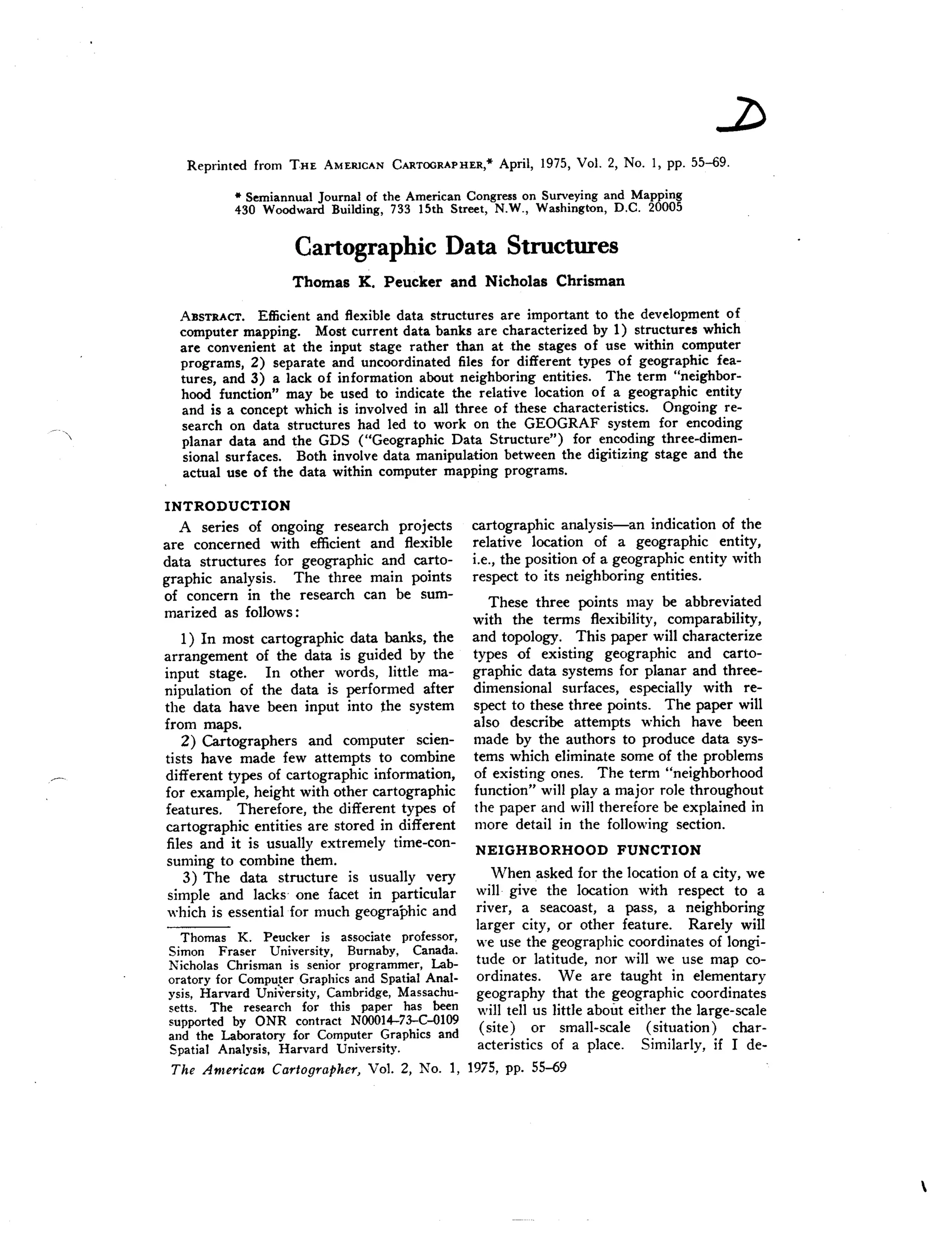
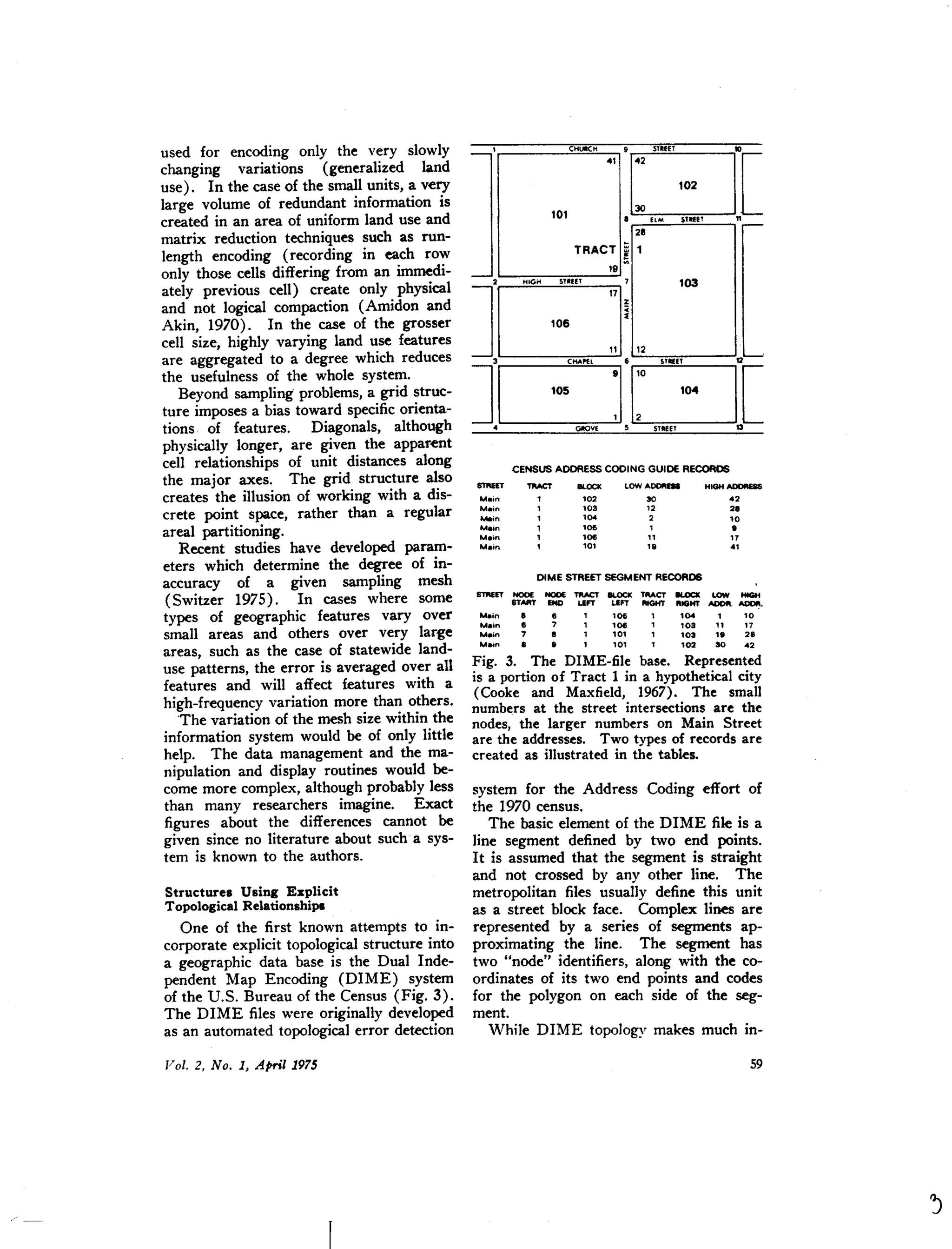
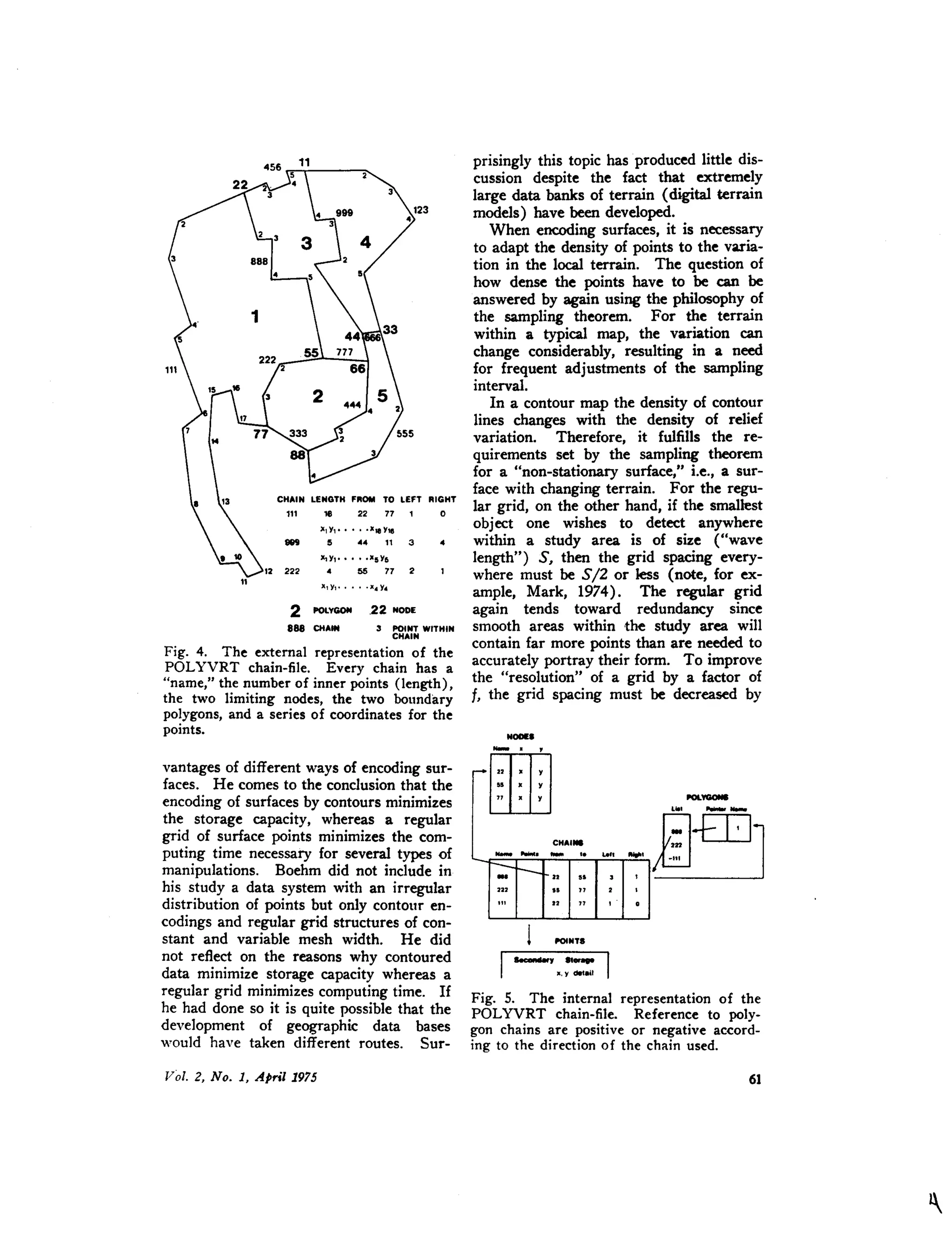
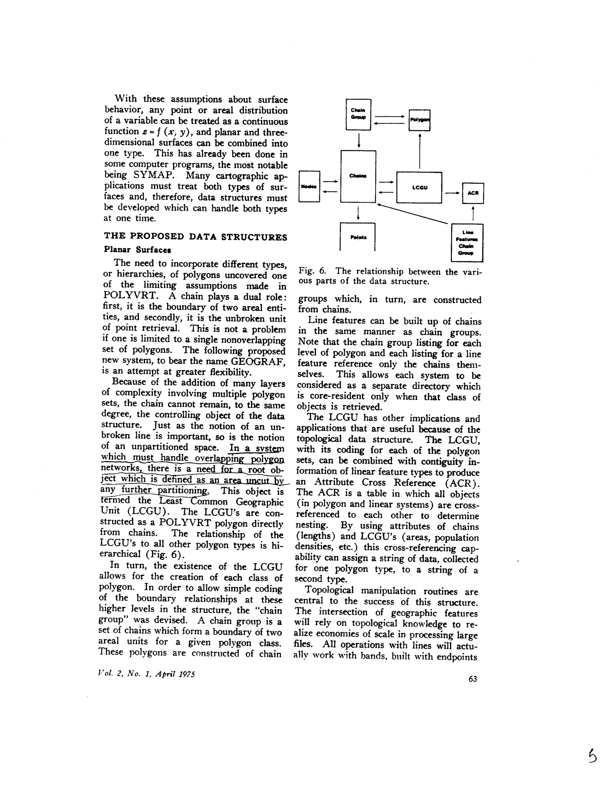
l'Fig. 7. The GDS-first data structure. The
illustration shows the points on the surface
with their links to neighbors (edges). The
external representation is shown by the
neighborhood relationships. The internal
representation is composedof the point-file
and the pointer-file.
two types: (a) sets of irregularly-distri-
buted points which were digitized with the
understanding that every point is signif-
icant, and (b) sets of regularly or irregu-
larly-distributed points where it is known
that a number of points are redundant and
can be eliminated from the set, e.g., regular
grids of points and encoded contours.
The first type of data set is linked by
some type of triangulation. At least two
approaches exist. The first (Dueppe and
Gottschalk, 1970) creates all possible links,
chooses the shortest, and eliminates all
links which intersect the shortest. This
procedure is repeated with the next short-
est links until no links intersect. The re-
sult is the set of links with the minimum
cumulative distance between neighboring
points.
The ~rocedure has one disadvantage:
since(~ ) links have to be created, the num-
ber of points is therefore limited to
only several hundred. The first step in
our approach therefore limits the links to
a number of "potential neighbors," among
which the shortest link is chosen and in-
tersected with all other links originating
in these potential neighbors. This pro-
cedure limits the number of tests for in-
n'm
2
tersections of links to less than - ••.-
where m is the number of potential neigh-
bors, an arbitrary number between 8 and
14 depending on the density variation of
these points. The procedure does not
guarantee, however, that only triangles are
constructed; polygons with more than
three sides can result, although they are
relatively rare. The check for such poly-
gons and their elimination is very easy and
fast.
The second possibility is to create a
triangulated structure through use of
Thiessen polygons. A published solution
(Rhynsburger, 1973) intersects for every
point the links to every other point midway
and chooses the smallest polygon created
I
_. CHA. I
~COID~oImJIIL ..•....• ........ER. CHAIN••••• _
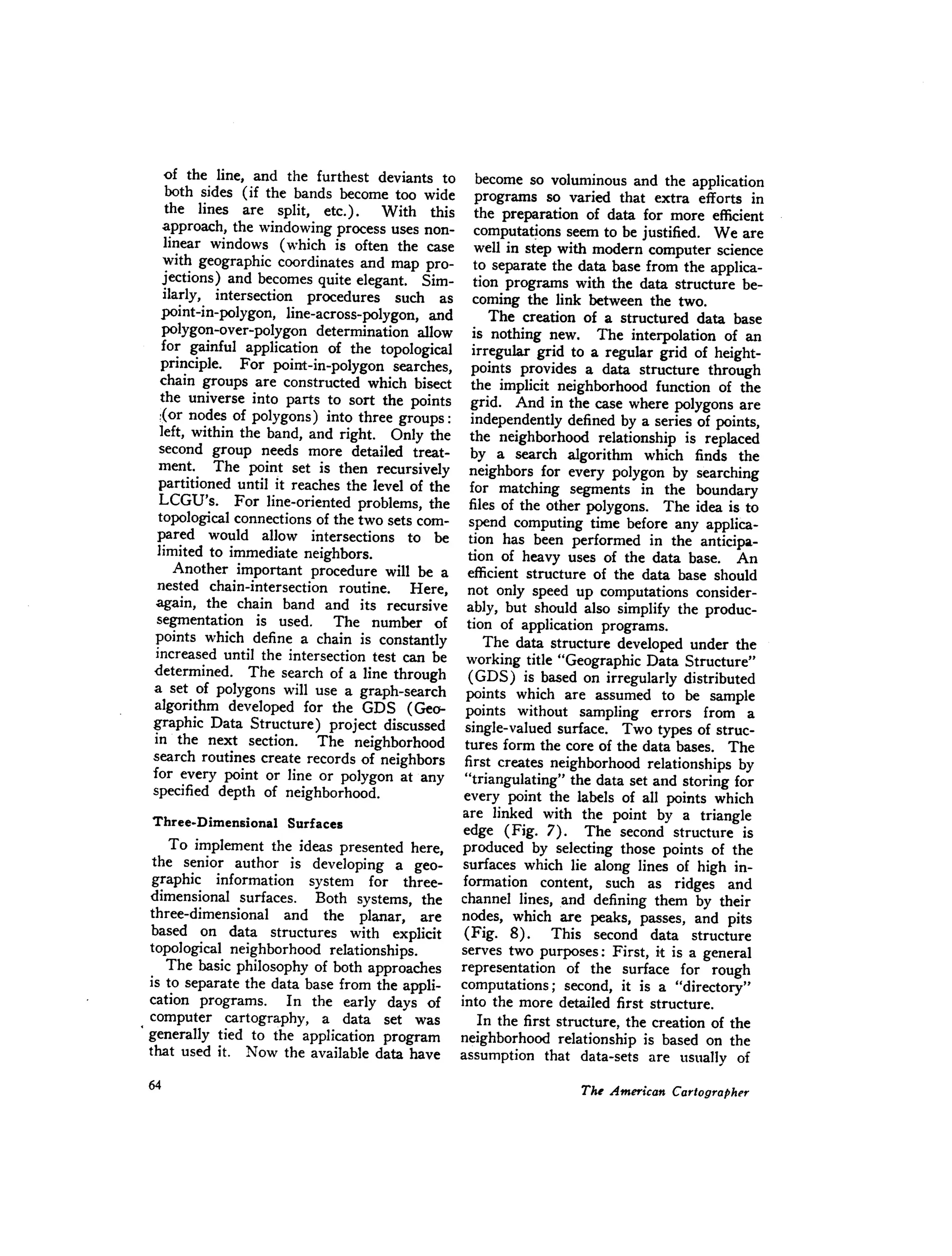
[[]]-D D[ _.T ~TA ~ROCT~ JFig. 8. The GDS-second data structure.
Both the node-file and the chain-file have
access to the first data structure, the node-
file directly and the chain-file through a
chain-pointer-file.

12. by the perpendiculars. Every point which
contributes to the Thiessen polygon is a
Thiessen neighbor. This procedure can
again be simplified by the assumption of a
limited set of "potential neighbors." The
same checking routines as above have to
be applied.
Another approach which limits the num-
ber of necessary tests, but is mathemat-
ically correct at the same time, has been
developed within the project by Kurt
Brassel at Harvard University. The pro-
cedure is based on "fields of potential
neighbors" which converge very rapidly.
The alternative to triangulation is three-
dimensional generalization, i.e., to select
from a set of points those which define the
structure with the least deviation from the
original surface. The basic concept, de-
veloped by Randolph Franklin of Harvard
University and T. K. Peucker, is to ap-
proximate the surface of a series of tri-
angles through a selected set of points,
where each additional point included into
the set is the one which deviates the most
from the approximated triangles until the
deviations are below a given value (see
Peucker, 1974).
In both cases, the triangulation and gen-
eralization of the surface, the result is a
"linked list" of surface points. The term
linked list means that points are linked with
one another through pointers. In other
words, a point is not only identified by its
x, y, z coordinates, but also by a list of the
labels of the points which form edges of
triangles with the point. In our case each
record consists of the x, y, z coordinates of
a point and a reference to the start of the
pointers to the neighbors in a pointer list.
The reason for not having the neighbor-
hood pointers with the point record is that
the number of points varies considerably
(Mark, 1974). Since the record has to be
long enough to include all possible num-
bers of neighbors, large parts of the pointer
sections would be empty most of the time.
The pointers are sorted, starting with the
pointer the least East of North of a point
(Fig. 7).
The use of this type of data-structure is
very simple and efficient. For every search
(profile, contour, etc.) a criterion for edge-
intersection is developed. For contouring,
for example, the critical question is
whether one point of the edge is above the
contour level and the other below. A start
is found and one point of the edge is con-
sidered a reference point and the other a
subpoint. The next subpoint is found by
looking up the next neighbor in the pointer
list. If the test is positive, the intersection
is performed and the process repeated. If
the test is negative, the reference and sub-
points are switched and the process re-
peated.
Other procedures are equally simple.
To find a triangle, for example, one has
only to have a reference and a subpoint.
The third point is the next label in the
pointer list of the reference point after the
subpoint. To find all triangles one goes
through the total pointer list leaving -out
all those edges connecting reference points
with subpoints with a smaller label since
they would create triangles which had
been treated when the subpoint was a
reference point.
Although the first data structure, as
presented above, seems to be efficient in
terms of storage capacity, it does not pro-
vide easy access to the data base which is
often very large. It is for this reason
that we are developing the second data
structure to represent the general structure
of the surface and to serve as a directory
to reach into the first data base (Pfaltz,
1975) (Fig. 8).
The first step in the creation of the
second data structure is to find the ridge,
channel, and break lines on the surface. If
one labels the highest point for every tri-
angle, the unlabeled points are members
of the channel line, at least on smooth
surfaces. A subsequent search routine
deals with the irregularities. Points along
ridges are found by eliminating the lowest
point of every triangle, using a routine
developed for a regular grid by D. M.
Douglas. The detection of break lines is
somewhat more difficult.
Some theoretical studies of surfaces by
Warntz (1966) show that ridge lines and
channel lines cross at passes, a useful point

13. of information relative to the development
of the second data structure. Practical
considerations suggest that in terrain and
other surfaces, this regularity is not always
present.
Once the topological structure is at hand,
it can be used as a directory into the first
structure. The line is therefore treated
as a chain similar to the chain of the
POLYVRT system. The nodes of the
chain are the peaks, passes, pits, and other
endpoints of chains on the surfaces. These
points are stored with their coordinates
and the names of the chains which termi-
nate at the nodes. The chains are stored
with the labels of the nodes and pointers
into the chain lists which consist of labels
of points in the first data structure (note
that here the chain structure differs from
that of POLYVRT).
A third component of the "Geographic
Data Structure" should be mentioned since
it illustrates very well the logical. a'dapta-
tion of a computer problem solution to
geographical data. The problem at hand
is the partitioning of the data set. Since
with large data sets only portions can be
kept in fast memory, the data base is seg-
mented into "pages" which are brought
into memory as units. For the "Geo-
graphic Data Structure" the paging sys-
tem can solve several problems inherent
in a complex geographic information sys-
tem.
The boundaries of "patches," as we call
the areal extension of a "page," are chains
already defined for the second structure.
Since detail along the chain is of no topo-
logical interest, the density of points along
the chain can differ for its two sides. In
other words, the density of triangles can
change from patch to patch. This allows
for very efficient data encoding even in
terrain with sudden changes in the sur-
face behavior as at the change from a
mountainous area into a plain (Peucker,
19i2) .
Another advantage of the paging-system
is the ease of including topographic and
planar information. Linking point, line,
and areal data to the triangulated points
would lead to high definitional redundancy.
The secondary structure could lead to am-
biguities where the terrain is very elon-
gated. Since an attempt has been made to
keep the shape of the patches as compact
as possible, the combination of non-terrain
data with patch boundaries seems to be
most appropriate.
Since the patch boundaries are again
chains, another virtue comes to light: The
patches can be treated as polygons of the
POLYVRT system with little difficulty.
This link between the two systems lends
hope that eventually they may be merged.
It is an appropriate question to ask what
such a data structure as the GDS will be
able to accomplish. A number of display
routines have already been developed
(Cochrane, 1974) and a series of proce-
dures for surface analysis based on heuris-
tic searches are underway (Fig. 9). Since
both levels of data structure are graphs,
we will be able to rely on many of the de-
velopments connected with operations re-
search, specifically network analysis, for
the manipulative treatment of the data.
As both systems, GDS and GEOGRAF,
have topological structures, it is possible
to merge the two. The creation of poly-
gons from points is the major link from
the GDS project to GEOGRAF. The
creation of a set of centroids for polygons
allows the conversion in the opposite direc-
tion. This way, surfaces can be treated as
polygonal sets and can be displayed and
manipulated by the routines of GEO-
GRAF. Conversely, polygonal data can
be treated as surfaces for GDS. The
neighborhood routines are what make the
project useful in quantitative geography
and planning. Neighborhood searches are
extremely expensive without the topologi-
cal data structure, but they are usually a
most important part of urban and environ-
mental analyses once a general overview is
obtained from the data.
Although basic research and application
development are two sides of one coin and
must go together to obtain lasting results,
this paper has concentrated on the theo-
retical parts of the project since their de-
velopment is ahead of the application rou-
tines, a fact which should be expected.

14. Contouring
Block Diagram
Sh8ded Contours
Inclined Contoura
Viaibility Teat
Radar Imalle
Fig. 9. The problem flow for GDS from the data base, via the
chains for the two types of data structures, to their application.
REGULAR GRID
IGENERALiZA TlON
TRIANGULATED
IRREGULAR GRID
Firat Data Structure
!
The quintessence of the research so far is
the hypothesis that topologically-structured
data bases of three-dimensional and planar
surfaces can result in reduced efforts in
the development and execution of applica-
REFERENCES
Amidon, E. L. and G. S. Aiken (1970), "Al-
gorithmic Selection of the Best Method for
Compressing Map Data Strings," Communica-
NOns of the Association for Computing Ma-
chinery, Vol. 14, pp. 769-774.
THEORY OF
SURFACE SPECiFIC
POINTS AND LINES
SURFACE SPECIFIC
POINTS AND LINES
Second Data Structure
HEURISTIC SEARCH
1SEARCH
Profile Search
Geographic Diaorientatlon
Oplimum Search
Neighborhood Analyaia
tion routines. We have some indication
that the hypothesis is correct; the real test
will come when the bulk of the application
routines is completed.
Arms, A. (1970), MAP/MODEL System: Sys-
tem Description and User's Guide, Bureau of
Governmental Research and Service, Univer-
sity of Oregon, 59 pp.
Boehm, B. M. (1967), "Tabular Representation

15. of Multivariate Functions with Applications
to Topographic Modelling," Proceedings, 22nd
National Conference, Association for Comput-
ing Machinery, pp. 403-415.
Brandstaetter, L. (1957), "Exakte Schichtlinien
und Topographische Gelaendedarstellung,"
Oesterreichische Zeitschrift fuer Vermessungs-
wesen, Sonderheft 18, Wien, 90 pp.
Cochrane, Douglas (1974), "Cartographic Dis-
play Operations on Surface Data Collected in
an Irregular Structure," M.A. thesis, Simon
Fraser University.
Cooke, D. F. and W. F. Maxfield (1967), "The
Development of a Geographic Base File and
Its Uses for Mapping," Urban and RegiOJlal
Information Systems for Social Programs, Pa-
pers from the 5th Annual Conference of the
Urban and Regional Information System As-
sociation, pp. 207-218.
Douglas, David H. (1973), "BNDRYNET,"
Peucker, T. K. (ed.) , The Interactive Map in
Urban Research, Final Report After Year One,
University of British Columbia.
Dueppe, R. D. and H. ]. Gottschalk (1970),
"Automatische Interpolation von Isolinien bei
willkuerlich verteilten Stuetzpunkten," Allge-
meine Vermessungs-Nachrichten, Vol. 129, No.
10 (Oct.), pp. 423-426.
Grist, M. W. (1972), "Digital Ground Models:
An Account of Recent Research," Photogram-
metric Record, Vol. 70, No.4 (Oct.), pp. 424-
441.
Heiskanen, W. A. and H. Moritz (1967), Phys-
ical Geodesy, W. H. Freeman, San Francisco,
Chapter 7.
Holroyd, M. T. and B. K. Bhattacharyya
(1970), Automatic Contouring of Geophysical
Data Using Bicubic Spline Interpolation, Geo-
logical Survey of Canada, Paper No. 70-55.
Hsu, M. L., et al., (1975), "Computer Applica-
tions in Land Use Mapping and the Minnesota
Land Management Information System," Da-
vis, J. c. and M. McCullagh (eds.), DisPlay
and Analysis of Spatial Data, New York, John
Wiley and Sons.
Junkins, ]. L., G. M. Miller and J. R. Jancaitis
(1973), "A Weighting Function Approach to
Modelling of Irregular Surfaces," Journal of
Geoph:!o,sicalResearch, Vol. 78, No. 11 (Apr.),
pp. 1794-1803.
Kraus, K. (1973), "A General Digital Terrain
Model," translation from an article in Acker-
mann, F. (1973), Numerische Photogram-
meme, Sammlung Wiechmann, Neue Folge,
Buchreihe. Bd. 5, Karlsruhe.
Laboratory for Computer Graphics and Spatial
Analysis, Harvard University (1974), POLY-
VRT Manual, Cambridge, Mass.
Mark, David M. (1974), "A Comparison of
Computer-based Terrain Storage Methods
With Respect to Evaluation of Certain Geo-
morphometric Measures," M.A. thesis, Uni-
versity of British Columbia.
Morse, S. P. (1968), "A Mathematical Model
for the Analysis of Contouring Line Data,"
Journal of the Association for Computing Ma-
chinery, Vol. IS, No.2, pp. 205-220.
Nake, F. and T. K. Peucker (1972), The Inter-
active Map in Urba" Research, Report after
Year 0,." University of British Columbia.
Nordbeck, S. and B. Rystedt (1970), "Isarithmic
Maps and the Continuity of Reference Interval
Functions," Geografiska Annaler, Vol. 52, Ser.
B., pp. 92-123.
Peucker, T. K. (1972), Computer Cartography,
Association of American Geographers, College
Geography Commission, Resource Paper No.
17, Washington, D.C.
Peucker, T. K. (ed.) (1973), The Interactive
Map in Urban Research, Final Report After
Year One," University of British Columbia.
Peucker, T. K. (1974), Geographical Data
Structures Report After Year One, Simon
Fraser University.
Pfaltz, J. L. (1975), "Surface Networks," Geo-
graphical Analysis (forthcoming).
Rhynsburger, D. (1973), "Analytic Delineation
of Thiessen Polygons," Geographical Analysis,
Vol. 5, No.2 (Apr.), pp. 133-144.
Rosenfeld, A. (1969), Picture Processing by
Computer, New York, Academic Press.
Schmidt, W. (1969), "The Automap System,"
Surveying and Mapping, Vol. 29, No. 1
(Mar.), pp. 101-106.
Shepard, D. (1968), "A Two-Dimensional Inter-
polation Function for Irregularly Spaced
Data," Proceedings, 23rd National Conference,
Association for Computing Machinery, pp. 517-
524.
Sima, J. (1972), "Prinzipien des CS digitalen
Gelaendemodells," Vermessungstechnik, Vol.
20, No.2, pp. 48-51.
Switzer, P. (1975) , in: "Sampling of Planar
Surfaces," Davis, J. C. and M. McCullagh
(eds.) , Display and Analysis of Spatial Data,
John Wiley and Sons, New York.
Tobler, W. R. (1969), "Geographical Filters and
their Inverses," GeograPhical Analysis, Vol. 1,
pp. 234-253.
Warntz, W. (1%6), "The Topology of Socio-
Economic Terrain and Spatial Flows," Papers
of the Regional Science Association, Vol. 17,
pp. 47~1. •