
More Related Content
What's hot
What's hot (19)
Viewers also liked
Viewers also liked (14)
Similar to A comparative analysis of predictve data mining techniques4
Similar to A comparative analysis of predictve data mining techniques4 (20)
Recently uploaded
Recently uploaded (20)
A comparative analysis of predictve data mining techniques4
- 1. Partial Least Square Regression PLS-Regression Hervé Abdi1 1 Overview P LS regression is a recent technique that generalizes and combines features from principal component analysis and multiple regres- sion. Its goal is to predict or analyze a set of dependent variables from a set of independent variables or predictors. This predic- tion is achieved by extracting from the predictors a set of orthog- onal factors called latent variables which have the best predictive power. P LS regression is particularly useful when we need to predict a set of dependent variables from a (very) large set of indepen- dent variables (i.e., predictors). It originated in the social sciences (specifically economy, Herman Wold 1966) but became popular first in chemometrics (i.e., computational chemistry) due in part to Herman’s son Svante, (Wold, 2001) and in sensory evaluation (Martens & Naes, 1989). But PLS regression is also becoming a tool of choice in the social sciences as a multivariate technique for non- experimental and experimental data alike (e.g., neuroimaging, see Mcintosh & Lobaugh, 2004; Worsley, 1997). It was first presented 1 In: Neil Salkind (Ed.) (2007). Encyclopedia of Measurement and Statistics. Thousand Oaks (CA): Sage. Address correspondence to: Hervé Abdi Program in Cognition and Neurosciences, MS: Gr.4.1, The University of Texas at Dallas, Richardson, TX 75083–0688, USA E-mail: herve@utdallas.edu http://www.utd.edu/∼herve 1
- 2. Hervé Abdi: PLS-Regression as an algorithm akin to the power method (used for computing eigenvectors) but was rapidly interpreted in a statistical framework. (see e.g., Phatak, & de Jong, 1997; Tenenhaus, 1998; Ter Braak & de Jong, 1998). 2 Prerequisite notions and notations The I observations described by K dependent variables are stored in a I × K matrix denoted Y, the values of J predictors collected on these I observations are collected in the I × J matrix X. 3 Goal of PLS regression: Predict Y from X The goal of PLS regression is to predict Y from X and to describe their common structure. When Y is a vector and X is full rank, this goal could be accomplished using ordinary multiple regres- sion. When the number of predictors is large compared to the number of observations, X is likely to be singular and the regres- sion approach is no longer feasible (i.e., because of multicollinear- ity). Several approaches have been developed to cope with this problem. One approach is to eliminate some predictors (e.g., us- ing stepwise methods) another one, called principal component regression, is to perform a principal component analysis (PCA) of the X matrix and then use the principal components (i.e., eigen- vectors) of X as regressors on Y. Technically in PCA, X is decom- posed using its singular value decomposition as X = S∆VT with: ST S = VT V = I, (these are the matriceds of the left and right singular vectors), and ∆ being a diagonal matrix with the singular values as diagonal el- ements. The singular vectors are ordered according to their corre- sponding singular values which correspond to the square root of 2
- 3. Hervé Abdi: PLS-Regression the variance of X explained by each singular vector. The left sin- gular vectors (i.e., the columns of S) are then used to predict Y us- ing standard regression because the orthogonality of the singular vectors eliminates the multicolinearity problem. But, the problem of choosing an optimum subset of predictors remains. A possible strategy is to keep only a few of the first components. But these components are chosen to explain X rather than Y, and so, noth- ing guarantees that the principal components, which “explain” X, are relevant for Y. By contrast, PLS regression finds components from X that are also relevant for Y. Specifically, PLS regression searches for a set of components (called latent vectors) that performs a simultane- ous decomposition of X and Y with the constraint that these com- ponents explain as much as possible of the covariance between X and Y. This step generalizes PCA. It is followed by a regression step where the decomposition of X is used to predict Y. 4 Simultaneous decomposition of predictors and dependent variables P LS regression decomposes both X and Y as a product of a com- mon set of orthogonal factors and a set of specific loadings. So, the independent variables are decomposed as X = TPT with TT T = I with I being the identity matrix (some variations of the technique do not require T to have unit norms). By analogy with PCA, T is called the score matrix, and P the loading matrix (in PLS regression the loadings are not orthogonal). Likewise, Y is estimated as Y = TBCT where B is a diagonal matrix with the “regression weights” as diagonal elements and C is the “weight matrix” of the dependent variables (see below for more details on the regression weights and the weight matrix). The columns of T are the latent vectors. When their number is equal to the rank of X, they perform an exact de- composition of X. Note, however, that they only estimate Y. (i.e., in general Y is not equal to Y). 3
- 4. Hervé Abdi: PLS-Regression 5 P LS regression and covariance The latent vectors could be chosen in a lot of different ways. In fact in the previous formulation, any set of orthogonal vectors span- ning the column space of X could be used to play the rôle of T. In order to specify T, additional conditions are required. For PLS regression this amounts to finding two sets of weights w and c in order to create (respectively) a linear combination of the columns of X and Y such that their covariance is maximum. Specifically, the goal is to obtain a first pair of vectors t = Xw and u = Yc with the constraints that wT w = 1, tT t = 1 and tT u be maximal. When the first latent vector is found, it is subtracted from both X and Y and the procedure is re-iterated until X becomes a null matrix (see the algorithm section for more). 6 A PLS regression algorithm The properties of PLS regression can be analyzed from a sketch of the original algorithm. The first step is to create two matrices: E = X and F = Y. These matrices are then column centered and normalized (i.e., transformed into Z -scores). The sum of squares of these matrices are denoted SS X and SS Y . Before starting the it- eration process, the vector u is initialized with random values. (in what follows the symbol ∝ means “to normalize the result of the operation”). Step 1. w ∝ ET u (estimate X weights). Step 2. t ∝ Ew (estimate X factor scores). Step 3. c ∝ FT t (estimate Y weights). Step 4. u = Fc (estimate Y scores). If t has not converged, then go to Step 1, if t has converged, then compute the value of b which is used to predict Y from t as b = tT u, and compute the factor loadings for X as p = ET t. Now subtract (i.e., partial out) the effect of t from both E and F as follows E = 4
- 5. Hervé Abdi: PLS-Regression E − tpT and F = F − btcT . The vectors t, u, w, c, and p are then stored in the corresponding matrices, and the scalar b is stored as a diagonal element of B. The sum of squares of X (respectively Y) explained by the latent vector is computed as pT p (respectively b 2 ), and the proportion of variance explained is obtained by dividing the explained sum of squares by the corresponding total sum of squares (i.e., SS X and SS Y ). If E is a null matrix, then the whole set of latent vectors has been found, otherwise the procedure can be re-iterated from Step 1 on. 7 PLS regression and the singular value decomposition The iterative algorithm presented above is similar to the power method (for a description, see Abdi, Valentin,& Edelman, 1999) which finds eigenvectors. So PLS regression is likely to be closely related to the eigen- and singular value decompositions, and this is indeed the case. For example, if we start from Step 1 which com- putes: w ∝ ET u, and substitute the rightmost term iteratively, we find the following series of equations: w ∝ ET u ∝ ET Fc ∝ ET FFT t ∝ ET FFT Ew. This shows that the first weight vector w is the first right singular vector of the matrix XT Y. Similarly, the first weight vector c is the left singular vector of XT Y. The same argument shows that the first vectors t and u are the first eigenvectors of XXT YYT and YYT XXT . 8 Prediction of the dependent variables The dependent variables are predicted using the multivariate re- gression formula as Y = TBCT = XBPLS with BPLS = (PT + )BCT (where PT + is the Moore-Penrose pseudo-inverse of PT ). If all the latent variables of X are used, this regression is equivalent to principal component regression. When only a subset of the latent variables is used, the prediction of Y is optimal for this number of predictors. 5
- 6. Hervé Abdi: PLS-Regression Table 1: The Y matrix of dependent variables. Wine Hedonic Goes with meat Goes with dessert 1 14 7 8 2 10 7 6 3 8 5 5 4 2 4 7 5 6 2 4 Table 2: The X matrix of predictors. Wine Price Sugar Alcohol Acidity 1 7 7 13 7 2 4 3 14 7 3 10 5 12 5 4 16 7 11 3 5 13 3 10 3 An obvious question is to find the number of latent variables needed to obtain the best generalization for the prediction of new observations. This is, in general, achieved by cross-validation tech- niques such as bootstrapping. The interpretation of the latent variables is often helped by ex- amining graphs akin to PCA graphs (e.g., by plotting observations in a t1 × t2 space, see Figure 1). 9 A small example 6
- 7. Hervé Abdi: PLS-Regression Table 3: The matrix T. Wine t1 t2 t3 1 0.4538 −0.4662 0.5716 2 0.5399 0.4940 −0.4631 3 0 0 0 4 −0.4304 −0.5327 −0.5301 5 −0.5633 0.5049 0.4217 Table 4: The matrix U. Wine u1 u2 u3 1 1.9451 −0.7611 0.6191 2 0.9347 0.5305 −0.5388 3 −0.2327 0.6084 0.0823 4 −0.9158 −1.1575 −0.6139 5 −1.7313 0.7797 0.4513 Table 5: The matrix P. p1 p2 p3 Price −1.8706 −0.6845 −0.1796 Sugar 0.0468 −1.9977 0.0829 Alcohol 1.9547 0.0283 −0.4224 Acidity 1.9874 0.0556 0.2170 7
- 8. Hervé Abdi: PLS-Regression Table 6: The matrix W. w1 w2 w3 Price −0.5137 −0.3379 −0.3492 Sugar 0.2010 −0.9400 0.1612 Alcohol 0.5705 −0.0188 −0.8211 Acidity 0.6085 0.0429 0.4218 Table 7: The matrix BPLS when 3 latent vectors are used. Hedonic Goes with meat Goes with dessert Price −1.0607 −0.0745 0.1250 Sugar 0.3354 0.2593 0.7510 Alcohol −1.4142 0.7454 0.5000 Acidity 1.2298 0.1650 0.1186 Table 8: The matrix BPLS when 2 latent vectors are used. Hedonic Goes with meat Goes with dessert Price −0.2662 −0.2498 0.0121 Sugar 0.0616 0.3197 0.7900 Alcohol 0.2969 0.3679 0.2568 Acidity 0.3011 0.3699 0.2506 We want to predict the subjective evaluation of a set of 5 wines. The dependent variables that we want to predict for each wine are its likeability, and how well it goes with meat, or dessert (as rated by a panel of experts) (see Table 1). The predictors are the price, the sugar, alcohol, and acidity content of each wine (see Table 2). The different matrices created by PLS regression are given in Tables 3 to 11. From Table 11 one can find that two latent vec- 8
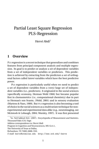
- 9. Hervé Abdi: PLS-Regression Table 9: The matrix C. c1 c2 c3 Hedonic 0.6093 0.0518 0.9672 Goes with meat 0.7024 −0.2684 −0.2181 Goes with dessert 0.3680 −0.9619 −0.1301 Table 10: The b vector. b1 b2 b3 2.7568 1.6272 1.1191 tors explain 98% of the variance of X and 85% of Y. This suggests to keep these two dimensions for the final solution. The exam- ination of the two-dimensional regression coefficients (i.e., BPLS , see Table 8) shows that sugar is mainly responsible for choosing a dessert wine, and that price is negatively correlated with the per- ceived quality of the wine, whereas alcohol is positively correlated with it (at least in this example . . . ). Looking at the latent vectors shows that t1 expresses price and t2 reflects sugar content. This in- terpretation is confirmed and illustrated in Figures 1a and b which display in (a) the projections on the latent vectors of the wines (matrix T) and the predictors (matrix W), and in (b) the correla- tion between the original dependent variables and the projection of the wines on the latent vectors. 10 Relationship with other techniques P LS regression is obviously related to canonical correlation, STATIS, and to multiple factor analysis. These relationships are explored in details by Tenenhaus (1998), Pagès and Tenenhaus (2001), and Abdi (2003b). The main originality of PLS regression is to preserve the asymmetry of the relationship between predictors and depen- 9
- 10. Table 11: Variance of X and Y explained by the latent vectors. Cumulative Cumulative Percentage of Percentage of Percentage of Percentage of Explained Explained Explained Explained 10 Variance for X Variance for X Variance for Y Variance for Y Latent Vector 1 70 70 63 63 2 28 98 22 85 3 2 100 10 95 Hervé Abdi: PLS-Regression
- 11. LV 2 2 5 2 3 Acidity 1 Hervé Abdi: PLS-Regression Hedonic LV1 Alcohol Meat Price 1 11 4 Dessert Sugar a b Figure 1: PLS-regression. (a) Projection of the wines and the predictors on the first 2 latent vectors (respectively matrices T and W). (b) Circle of correlation showing the correlation between the original dependent variables (matrix Y) and the latent vectors (matrix T).
- 12. Hervé Abdi: PLS-Regression dent variables, whereas these other techniques treat them sym- metrically. 11 Software P LS regression necessitates sophisticated computations and there- fore its application depends on the availability of software. For chemistry, two main programs are used: the first one called SIMCA - P was developed originally by Wold, the second one called the U N - SCRAMBLER was first developed by Martens who was another pio- neer in the field. For brain imaging, SPM, which is one of the most widely used programs in this field, has recently (2002) integrated a PLS regression module. Outside these domains, SAS PROC PLS is probably the most easily available program. In addition, interested readers can download a set of MATLAB programs from the author’s home page (www.utdallas.edu/∼herve). Also, a public domain set of MATLAB programs is available from the home page of the N - Way project (www.models.kvl.dk/source/nwaytoolbox/) along with tutorials and examples. From brain imaging, a special toolbox written in MATLAB (by McIntosh, Chau, Lobaugh, & Chen) is freely available from www.rotman-baycrest.on.ca:8080. And finally, a commercial MATLAB toolbox has also been developed by E IGEN - RESEARCH . References [1] Abdi, H. (2003a&b). PLS-Regression; Multivariate analysis. In M. Lewis-Beck, A. Bryman, & T. Futing (Eds): Encyclopedia for research methods for the social sciences. Thousand Oaks: Sage. [2] Abdi, H., Valentin, D., & Edelman, B. (1999). Neural networks. Thousand Oaks (CA): Sage. [3] Escofier, B., & Pagès, J. (1988). Analyses factorielles multiples. Paris: Dunod. [4] Frank, I.E., & Friedman, J.H. (1993). A statistical view of chemo- metrics regression tools. Technometrics, 35 109–148. 12
- 13. Hervé Abdi: PLS-Regression [5] Helland I.S. (1990). P LS regression and statistical models. Scan- divian Journal of Statistics, 17, 97–114. [6] Höskuldson, A. (1988). P LS regression methods. Journal of Chemometrics, 2, 211-228. [7] Geladi, P., & Kowlaski B. (1986). Partial least square regression: A tutorial. Analytica Chemica Acta, 35, 1–17. [8] McIntosh, A.R., & Lobaugh N.J. (2004). Partial least squares analysis of neuroimaging data: applications and advances. Neuroimage, 23, 250–263. [9] Martens, H, & Naes, T. (1989). Multivariate Calibration. Lon- don: Wiley. [10] Pagès, J., Tenenhaus, M. (2001). Multiple factor analysis com- bined with PLS path modeling. Application to the analysis of relationships between physicochemical variables, sensory profiles and hedonic judgments. Chemometrics and Intelli- gent Laboratory Systems, 58, 261–273. [11] Phatak, A., & de Jong, S. (1997). The geometry of partial least squares. Journal of Chemometrics, 11, 311–338. [12] Tenenhaus, M. (1998). La régression PLS. Paris: Technip. [13] Ter Braak, C.J.F., & de Jong, S. (1998). The objective function of partial least squares regression. Journal of Chemometrics, 12, 41–54. [14] Wold, H. (1966). Estimation of principal components and re- lated models by iterative least squares. In P.R. Krishnaiaah (Ed.). Multivariate Analysis. (pp.391-420) New York: Acad- emic Press. [15] Wold, S. (2001). Personal memories of the early PLS develop- ment. Chemometrics and Intelligent Laboratory Systems, 58, 83–84. [16] Worsley, K.J. (1997). An overview and some new developments in the statistical analysis of PET and fMRI data. Human Brain Mapping, 5, 254–258. 13