Latin hypercube sampling

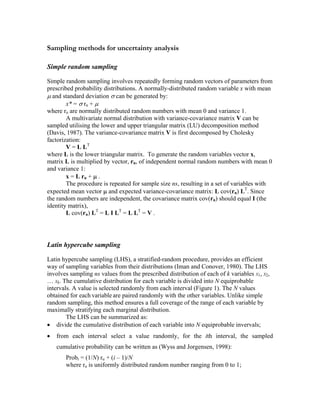
1. Sampling methods for uncertainty analysis
Simple random sampling
Simple random sampling involves repeatedly forming random vectors of parameters from
prescribed probability distributions. A normally-distributed random variable x with mean
µ and standard deviation σ can be generated by:
x* = σ rn + µ
where rn are normally distributed random numbers with mean 0 and variance 1.
A multivariate normal distribution with variance-covariance matrix V can be
sampled utilising the lower and upper triangular matrix (LU) decomposition method
(Davis, 1987). The variance-covariance matrix V is first decomposed by Cholesky
factorization:
V = L LT
where L is the lower triangular matrix. To generate the random variables vector x,
matrix L is multiplied by vector, rn, of independent normal random numbers with mean 0
and variance 1:
x = L rn + µ .
The procedure is repeated for sample size ns, resulting in a set of variables with
expected mean vector µ and expected variance-covariance matrix: L cov(rn) LT
. Since
the random numbers are independent, the covariance matrix cov(rn) should equal I (the
identity matrix),
L cov(rn) LT
= L I LT
= L LT
= V .
Latin hypercube sampling
Latin hypercube sampling (LHS), a stratified-random procedure, provides an efficient
way of sampling variables from their distributions (Iman and Conover, 1980). The LHS
involves sampling ns values from the prescribed distribution of each of k variables X1, X2,
… Xk. The cumulative distribution for each variable is divided into N equiprobable
intervals. A value is selected randomly from each interval (Figure 1). The N values
obtained for each variable are paired randomly with the other variables. Unlike simple
random sampling, this method ensures a full coverage of the range of each variable by
maximally stratifying each marginal distribution.
The LHS can be summarized as:
• divide the cumulative distribution of each variable into N equiprobable invervals;
• from each interval select a value randomly, for the ith interval, the sampled
cumulative probability can be written as (Wyss and Jorgensen, 1998):
Probi = (1/N) ru + (i – 1)/N
where ru is uniformly distributed random number ranging from 0 to 1;

2. • transform the probability values sampled into the value x using the inverse of the
distribution function F-1
:
x = F-1
(Prob) ;
• the N values obtained for each variable x are paired randomly (equally likely
combinations) with the ns values of the other variables.
The method is based on the assumption that the variables are independent of each
other, but in reality most of the input variables are correlated to some extent. Random
pairing of correlated variables could result in impossible combinations, furthermore
independent variables tend to bias the uncertainty.
0
0.2
0.4
0.6
0.8
1
-2 -1 0 1 2
x1
CumulativeProbability
0
0.2
0.4
0.6
0.8
1
-2 -1 0 1 2
x2
CumulativeProbabilit
Fig. 1. Example of LHS: Random stratified sampling of variables x1 and x2 at 5 intervals (Left)
and random pairing of sampled x1 and x2 forming a Latin hypercube (Right).
y
0
0.2
0.4
0.6
0.8
1
0 0.2 0.4 0.6 0.8 1
Probability x2
Probabilityx1
0
0.2
0.4
0.6
0.8
1
-2 -1 0 1 2
x1
CumulativeProbability
0
0.2
0.4
0.6
0.8
1
-2 -1 0 1 2
x2
CumulativeProbabilit
0
0.2
0.4
0.6
0.8
1
0 0.2 0.4 0.6 0.8 1
Probability x2
Probabilityx1
y

3. Inducing correlation in Latin hypercube sampling
Iman and Conover (1982) proposed a method for inducing correlation among the
variables by restricting the way the variables are paired based on the rank correlation of
some target values. The method is based on the Cholesky decomposition of the
correlation matrix. Suppose matrix X is composed of independent random variables with
correlation matrix I and C is the desired correlation matrix. Matrix C can be written as C
= P P’ where P is the lower triangular matrix. Similar to the simple random sampling,
multiplying vector x P’ yield random variables with correlation matrix C. Therefore the
objective is to rearrange the input variables close to the target correlation matrix. The
method is summarised as follows:
• generate matrix R using Latin hypercube sampling of k variables at sample size ns;
• calculate T, the correlation matrix of R;
• calculate the P lower triangular matrix of the target correlation matrix C using
Cholesky factorization C = P P’ and also Q the lower triangular matrix of T
T = Q Q’ ;
• solve to obtain matrix S such that STS’ = C, which is calculated from S = P Q-1
;
• calculate target correlation matrix R* = R S’, which has a correlation matrix equal to
C;
• rearrange the values of each variable in R so they have the same rank (order) as the
target matrix R*.
Stein (1987) also proposed a method for sampling dependent variables based on the
rank of a target multivariate distribution.
• obtain matrix R of k variables at sample size N using simple random sampling;
• define U the matrix with k columns and N rows containing the order or rank
corresponding to the target correlation matrix;
• obtain the Latin hypercube sample xij (i = 1, ..., N; j = 1, ..., k) by
u1
rij
ij j
u
x F
N
−
−⎛ ⎞
= ⎜
⎝ ⎠
⎟
With this shifting (transformation), the sampled values yield an approximately joint
distribution. See Pebesma and Heuvelink (1999) and Zhang and Pinder (2004) for more
detail description.

4. References
Cochran, W.G., 1977. Sampling Techniques, 3rd edn. John Wiley and Sons, New York.
Davis, M.W., 1987. Production of conditional simulations via the LU triangular decomposition of
the covariance matrix. Mathematical Geology 19, 91-98.
Iman, R.L., Conover, W.J., 1982. A distribution-free approach to inducing rank correlation
among input variables. Communications in Statistics B11, 311-334.
Iman, R.L., 1992. Uncertainty and sensitivity analysis for computer modeling applications. In:
Reliability Technology, The American Society of Mechanical Engineers 1992, (ed T.A.
Cruse), pp. 153-168. The American Society of Mechanical Engineers, New York.
McKay, M.D., Beckman, R.J., Conover, W.J., 1979. A comparison of three methods for selecting
values of input variables in the analysis of output from a computer code. Technometrics 21,
239-245.
Pebesma, E.J., Heuvelink, G.B.M., 1999. Latin hypercube sampling of Gaussian random fields.
Technometrics 41, 303-312.
Stein, M.L., 1987. Large sample properties of simulations using Latin hypercube sampling.
Technometrics, 29, 143-151.
Wyss, G.D., Jorgensen, K.H., 1998, A User’s Guide to LHS: Sandia’s Latin Hypercube Sampling
Software. Technical Report SAND98-0210. Sandia National Laboratories, Albuquerque, NM.
Zhang, Y., Pinder, G.F., 2004. Latin-Hypercube Sample-Selection Strategies for Correlated
Random Hydraulic-Conductivity Fields. Water Resources Research 39(8) SBH 11