Download to read offline
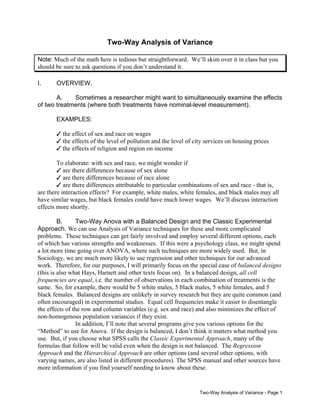
![Another useful partitioning is
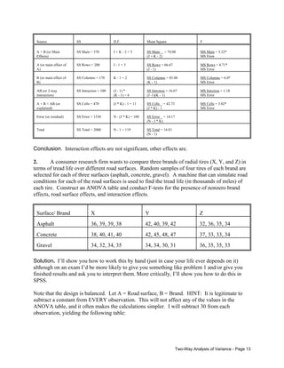
SS Cells = SS Explained = SS Main + SS Interaction = SS Total - SS Error
d.f. = JK - 1
When all cell frequencies are equal,
SS Cells = SS Columns + SS Rows + SS Interaction.
Finally, note that,
Total SS = SS Main + SS Interactions + SS Error = SS Explained + SS Error
d.f.= J - 1 + K - 1 + JK + 1 - J - K + N - JK = N - 1
Again, when all cell frequencies are equal,
Total SS = SS Columns + SS Rows + SS Interaction + SS Error.
E.
II.
When doing statistical inference, we assume that
T
for each treatment combination JK, the random error terms εijk are N(0, σ2); the variance σ2 is the same for each treatment combination.
T
the random error terms are independent
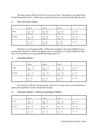
TESTS OF INTEREST:
A.
H0:
HA:
(τλ)jk = 0
(τλ)jk <> 0
for all j, k
for at least 1 j, k
This is a test of whether there are any interaction effects; the appropriate test statistic is
F (J -1)(K -1),N - JK =
SS Interaction/(J - 1)(K - 1) MS Interaction
=
SS Error/(N - JK)
MS Error
If the null hypothesis is true, F - F([J - 1][K - 1], N - JK)
B.
H0:
HA:
τ1 = τ2 =... = τJ = 0
At least 1 τj <> 0
Two-Way Analysis of Variance - Page 4](https://image.slidesharecdn.com/x61-140218124402-phpapp02/85/X61-4-320.jpg)
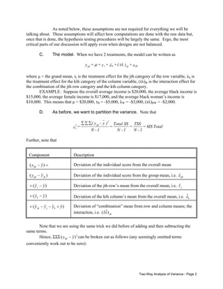
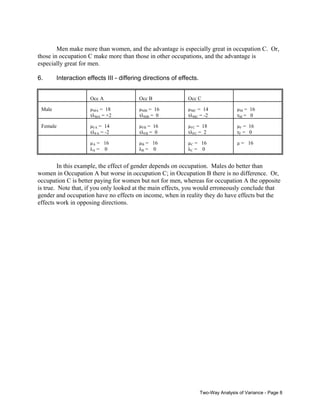
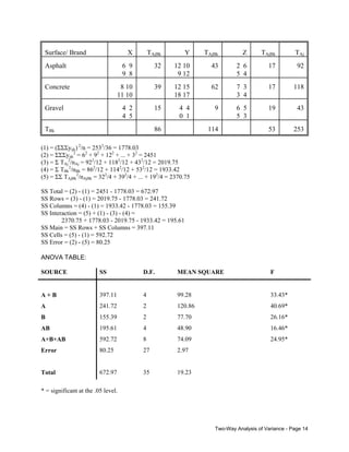
![This tests whether there are any row effects. The appropriate test statistic is
F J -1,N - JK =
SS Rows/(J - 1)
MS Rows
=
SS Error/(N - JK) MS Error
If the null hypothesis is true, F - F([J - 1], N - JK)
C.
H0:
HA:
λ1 = λ2 =... = λK = 0
At least 1 λk <> 0
This tests whether there are any column effects. The appropriate test statistic is
F K -1,N - JK =
SS Columns/(K - 1) MS Columns
=
SS Error/(N - JK)
MS Error
If the null hypothesis is true, F - F([K - 1], N - JK).
NOTE: The last two tests are primarily of interest if you conclude that interaction effects
are not significant. If, on the other hand, you conclude that the interaction effects do not equal
zero, then you know both treatments (i.e. the row and column effects) are significant.
D.
H0:
HA:
All τ’s and λ’s = 0
At least one τ or λ does not equal 0
This tests whether any of the main effects (i.e. row or column effects; or, non-interaction effects)
are nonzero. The appropriate test statistic is
F J + K - 2,N - JK =
SS Main/(J + K - 2) MS Main
=
SS Error/(N - JK) MS Error
If the null hypothesis is true, F - F([J + K - 2], N - JK).
E.
H0:
HA:
All τ’s, λ’s, and (τλ)’s = 0
At least one τ, λ, or (τλ) does not equal 0
This tests whether there are any effects at all. If the null hypothesis is true, then every
cell in the table will have the same true mean. The appropriate test statistic is
F JK -1,N - JK =
SS Cells/(JK - 1)
MS Cells
=
SS Error/(N - JK) MS Error
If the null hypothesis is true, F - F([JK - 1], N - JK).
Two-Way Analysis of Variance - Page 5](https://image.slidesharecdn.com/x61-140218124402-phpapp02/85/X61-5-320.jpg)
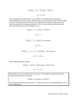
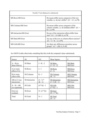
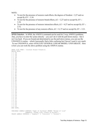
![IV.
Computational Procedures - Two-Way Anova – Balanced Designs
Let A = row variable, B = column variable, J = number of categories for A, K = number of
categories for B, TAj = the sum of the scores in group Aj, TBk = the sum of the scores in group Bk,
TAjBk is the sum of the scores for the observations which fall in both groups Aj and Bk (there are
J*K of these totals), nAj = number of observations in group Aj, nBk = number of observations in
group Bk, nAjBk is the number of observations which fall in both groups Aj and Bk. [NOTE:
While I will show you how to do the raw data calculations, in practice they are tedious enough
that I generally would not expect you to do them by hand, at least on an exam. You should know
how to do the other formulas, however, as they show how the different parts of the ANOVA
table are related to each other.]
Note that many (albeit not all) of the formulas for raw data calculations and Sums of Squares
assume a balanced design, i.e. all cell frequencies are equal for each possible combination of
values for the row and column variables. Computations are somewhat more complicated when
designs are not balanced. The Mean Square formulas and the F tests are accurate regardless of
whether the design is balanced or not.
Formula
Explanation
Raw Data Calculations (Balanced Design)
ˆ
(1) = (ΣΣΣyijk)2/n = Nµ 2
Sum all the observations. Square the result.
Divide by the total number of observations.
(2) = ΣΣΣyijk2
Square each observation. Sum the squared
observations.
(3) = Σ TAj2/nAj
Add up the values for the observations for group
A1. Square the result. Divide by the number of
observations in group A1. Repeat for each
category of A. Add the results for each of the J
groups together.
(4) = Σ TBk2/nBk
Add up the values for the observations for group
B1. Square the result. Divide by the number of
observations in group B1. Repeat for each
category of B. Add the results for each of the K
groups together.
(5) = ΣΣ TAjBk2/nAjBk
Add up the values for the observations which fall
in both group A1 and B1. Square this value, and
divide by nA1B1. Repeat for each of the J*K
combinations, and sum the results.
Two-Way Analysis of Variance - Page 9](https://image.slidesharecdn.com/x61-140218124402-phpapp02/85/X61-9-320.jpg)
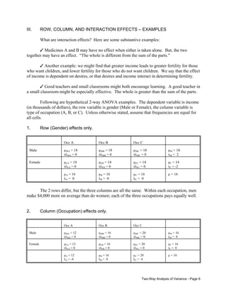
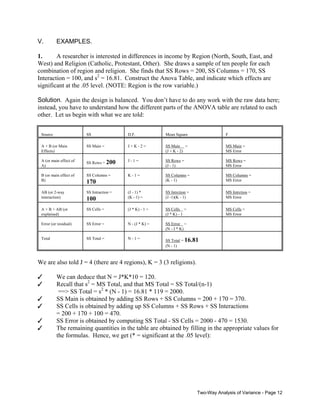
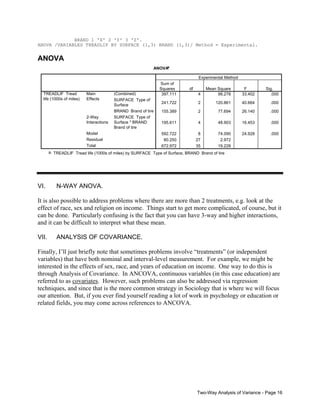
![Sums of Squares Calculations (Balanced Design)
SS Total = (2) - (1)
Total sum of squares
SS Rows = (3) - (1)
Row sum of squares. This is also sometimes
called SSA.
SS Columns = (4) - (1)
Column sum of squares. Also called SSB.
SS Interaction =
(5) + (1) - (3) - (4) =
SS Total - SS Rows - SS Columns - SS Error
= SS Total – SS Main – SS Error
Interaction sum of squares. Also called SSAB.
It may be easier to use the second formula.
SS Error = (2) - (5) = SS Total - SS Cells
Error sum of squares. It is analogous to SS
Within in one-way ANOVA. Also called SS
Residual.
SS Main = (3) + (4) – [2 * (1)] =
SS Columns + SS Rows =
SS Total – SS Error – SS Interaction
Main effects Sum of Squares. Also called
SSA+B
SS Cells = (5) - (1) =
SS Main + SS interaction =
SS Total - SS Error.
This is analogous to SS Between in one-way
ANOVA. Also called SS Explained.
Mean Square Calculations (Balanced or unbalanced)
MS Total = s2 =
SS Total/(n-1)
Remember that MS Total = s2
MS Rows =
SS Rows/(J-1)
Also called MSA.
MS Columns =
SS Columns/(K-1)
Also called MSB.
MS Interaction =
SS Interaction/((J-1)(K-1))
Also called MSAB
MS Main = SS Main/(J + K - 2)
Also called MSA+B
MS Cells =
SS Cells/((J*K)-1)
Also called MS Explained.
MS Error =
SS Error/ (n - J*K)
Also called MS Residual.
Two-Way Analysis of Variance - Page 10](https://image.slidesharecdn.com/x61-140218124402-phpapp02/85/X61-10-320.jpg)

1. This document provides an overview of two-way analysis of variance (ANOVA), which examines the effects of two treatments on an outcome. It describes how two-way ANOVA partitions variance and tests for row effects, column effects, interaction effects, and overall effects. 2. Examples are provided to illustrate row effects only, column effects only, both row and column effects, and four types of interaction effects. Interaction effects occur when the effect of one treatment depends on the level of the other treatment. 3. The assumptions of two-way ANOVA are that the error terms are normally distributed, independent, and have equal variances for each treatment combination. Hypothesis tests are described to examine row effects


![Lecture 5_Analysis of Variance [ANOVA].pptx](https://cdn.slidesharecdn.com/ss_thumbnails/lecture5analysisofvarianceanova-260107181555-9a697733-thumbnail.jpg?width=640&height=640&fit=bounds)


