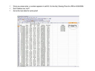
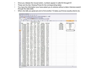
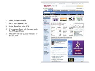
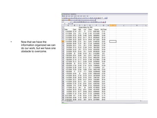
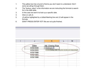
This document provides instructions for using the vLookup function in Excel to retrieve stock price data from a historical quotes table for JPMorgan Chase. It describes downloading historical stock price data to a spreadsheet, formatting and organizing the table, and then using vLookup to find the adjusted closing prices for specific dates by searching the date column and returning values from the adjusted closing price column. The vLookup formula is dragged down to automatically retrieve prices for multiple dates without having to retype the formula.

1. How to Use vLookup For Excel Presentation by Michael P. Nobile

2. The Scenario Your boss is doing some important research on JPMorgan Chase and she needs your help. She needs a general price history of the stock for the past 20 years in 5 year increments, including last years price. She asks you to pull up the figures for her and you immediately begin work.

3. Open your web browser Go to finance.yahoo.com In the Quote Box enter JPM A new screen loads with the day’s quote for JPMorgan Chase Click on “Historical Quotes” indicated by the red circle

4. A new screen loads with the historical quotes for JPM. Scroll to the bottom on this page as indicated by the red arrow.

5. Once you scroll to the bottom, click on “Download to Spreadsheet” as indicated by the red circle.

6. A grey box will appear. Select “Open with” and make sure Microsoft Office Excel is the program used for the purposes of this presentation. Click “OK”

7. Next, we need to organize the data for visual uniformity. With your pointer, select boxes A through G.

8. Click Center, once you have selected the boxes. Next, we need to resize the columns for the best fit of the data. Scroll your pointer over the border separating boxes A and B. A two-sided arrow with a larger vertical line in the center will appear. Double Click. The Column automatically adjusts to fit the data for that column. Do this for each column.

9. Next, we need to title this data table. Select the row labeled “1.” Once selected, right-click, and a menu will appear. Click Insert. A new row will be added to the table above row 1 and row 1 will become row 2.

10. Click into box A1. Click into the Formula Bar, as indicated by the red circle. Type “Quote History for JPM” Press Enter.

11. Select cells A1 through G1. Click the “Merge an Center” button indicated by the red circle. The title in A1 will merge and center across the selected cells. Your table should resemble mine.

12. Now that we have the information organized we can do our work, but we have one obstacle to overcome.

13. There is over 6,000 rows of data in our table of historical quotes. Without vLookup, doing the requested research would be time consuming and inefficient.

14. In cell J2 type the title “Dates,” italicize and underline it. For the most accurate information, we will use the Adjusted Close Price in Column G. In cell K1 type the title “Adj. Closing Price,” italicize and underline it. In the cells underneath your “ Dates ,” type the dates your boss needs quotes for.

15. In cell K3 type: =vlookup( A yellow box will appear right underneath the cell we are working in.

16. This yellow box has a bunch of terms you don’t seem to understand. Don’t worry we will go through them. The “lookup_value” is the information we are instructing the formula to search for in the data table. In this case we want it to look up a specific date. Click on cell J3. J3 will be highlighted by a dotted-flashing line and J3 will appear in the formula. DON’T PRESS ENTER YET! We are not quite finished.

17. Instead, enter a comma with no spaces before or after. “ table_array” stands for the data table we are using to search for the needed information. In this case it is the Quote History for JPM. To select our table, click on box A and the entire data table will automatically be selected by Excel and highlighted by a dotted flashing line. The table will be added to the formula represented as A:G. Enter another comma right after.

18. The “col_index_num” is the column where the data we need is located. This will allow the formula to correspond the dates we entered to the data in the selected column. The Adjusted Closing Price is represented in Column G with the title Adj Close. Column G is the seventh column in our data table. Right after our next comma type the number 7 and another comma; remember, no spaces.

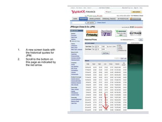
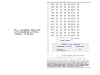
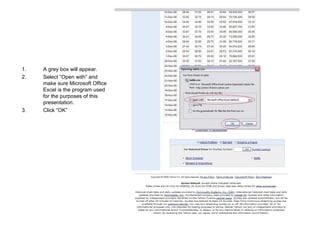
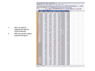
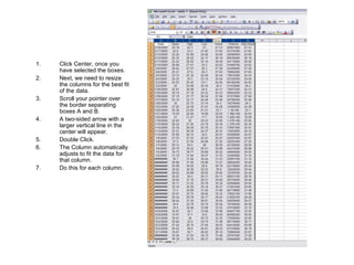
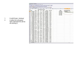
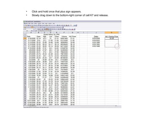
19. The last term in our yellow box is “[range_lookup]” which defines if we want an exact match of our dates or ones that come close to it. For an exact match of our dates we need to type “False” and and “)”. Press enter. If we type “True” we will not get the data we need and the formula will have too many dates that have a probable match.

20. Once you press enter, a number appears in cell K3. It’s the Adj. Closing Price for JPM on 6/30/2008. Don’t believe me, huh? Go to the next slide for some proof.

21. Row 163 has the price quote for 6/30/2008. If you look across to the Adj. Closing Price, you see the number 33.26. The same number that showed up in cell K3 after we typed our vLookup formula. Now we know our vLookup formula is working. Let’s find out the rest of the needed prices.

22. Now, your thinking we have to retype the entire vLookup formula all over again; but, we actually don’t have to. Select cell K3 and move the pointer over the bolded bottom-right corner of the cell. The pointer will change to a plus sign.

23. Click and hold once that plus sign appears. Slowly drag down to the bottom-right corner of cell K7 and release.

24. Once you release the mouse button, numbers appear in cells K4 through K7. These are the Adj. Closing Prices for the corresponding dates. You have the information your boss asked you to retrieve without a labor intensive search through the data table. When she tells you great job and to find another 10 dates you’ll know exactly what to do.