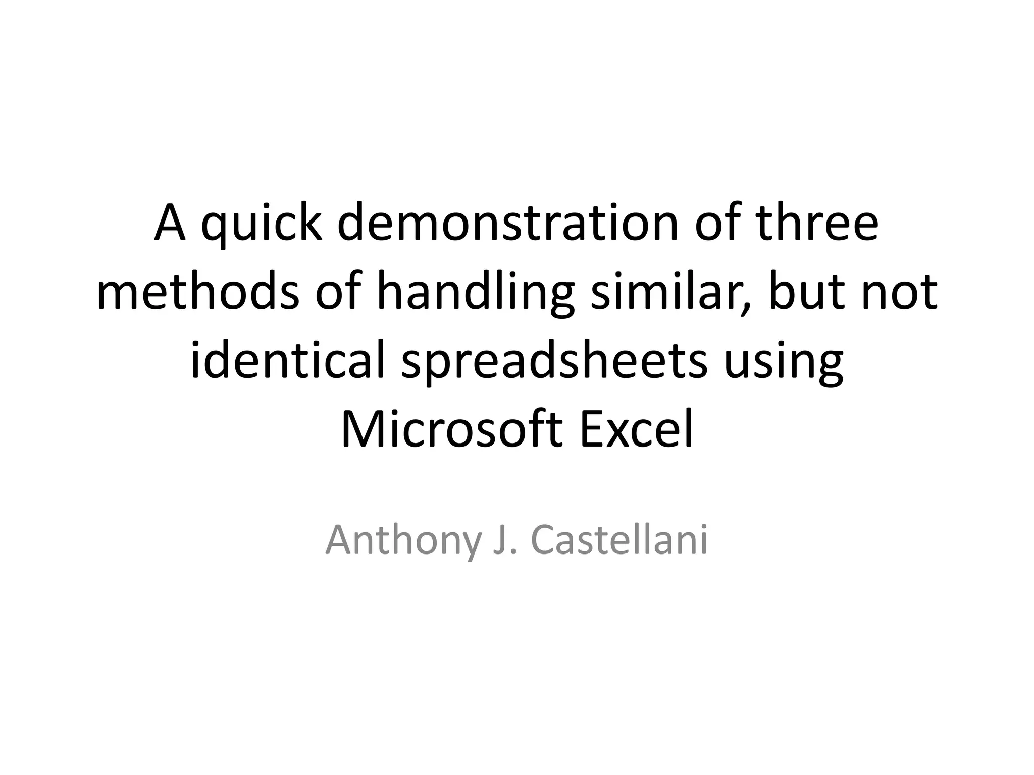
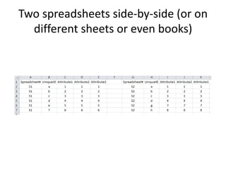
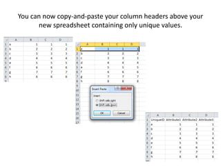
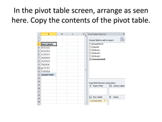
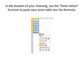
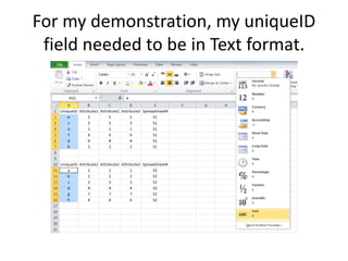
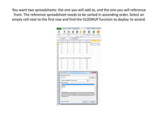
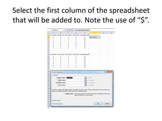
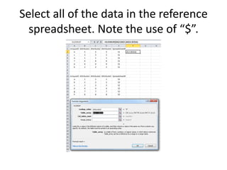
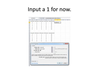
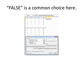
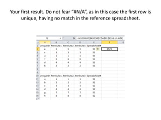
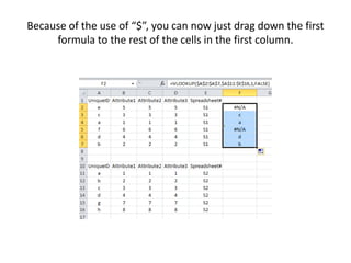
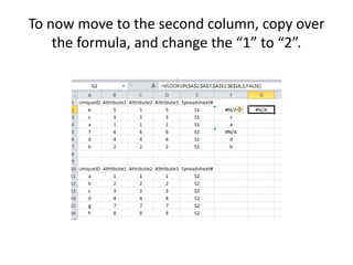
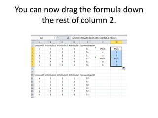
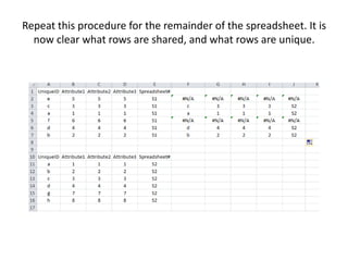
This document demonstrates three methods for handling similar but not identical spreadsheets in Microsoft Excel: 1) Copying the spreadsheets together and using tools to highlight duplicate values 2) Using a pivot table to arrange the data and identify unique values 3) Using VLOOKUP formulas to reference values between spreadsheets and identify shared and unique rows

1. A quick demonstration of three
methods of handling similar, but not
identical spreadsheets using
Microsoft Excel
Anthony J. Castellani

2. METHOD 1
Quick visualization

3. Two spreadsheets side-by-side (or on
different sheets or even books)

4. Copy the two spreadsheets into one block, highlight a column of
unique values, and use the “Duplicate Values” tool

5. METHOD 2
Pivot Tables

6. With the two spreadsheets copied together, add a column containing the
rows concatenated together. Use a symbol not otherwise found in the data to
separate values. Select the “PivotTable” tool.

7. In the pivot table screen, arrange as seen
here. Copy the contents of the pivot table.

8. In the location of your choosing, use the “Paste Values”
function to paste your pivot table less the formulas.

9. With your data still highlighted, use the “Text to Columns” tool.
Follow the wizard steps seen on the next slides.

10. Wizard continued

11. Wizard continued

12. You can now copy-and-paste your column headers above your
new spreadsheet containing only unique values.

13. METHOD 3
VLOOKUP

14. For my demonstration, my uniqueID
field needed to be in Text format.

15. You want two spreadsheets: the one you will add to, and the one you will reference
from. The reference spreadsheet needs to be sorted in ascending order. Select an
empty cell next to the first row and find the VLOOKUP function to deploy its wizard.

16. Select the first column of the spreadsheet
that will be added to. Note the use of “$”.

17. Select all of the data in the reference
spreadsheet. Note the use of “$”.

18. Input a 1 for now.

19. “FALSE” is a common choice here.

20. Your first result. Do not fear “#N/A”, as in this case the first row is
unique, having no match in the reference spreadsheet.

21. Because of the use of “$”, you can now just drag down the first
formula to the rest of the cells in the first column.

22. To now move to the second column, copy over
the formula, and change the “1” to “2”.

23. You can now drag the formula down
the rest of column 2.

24. Repeat this procedure for the remainder of the spreadsheet. It is
now clear what rows are shared, and what rows are unique.

25. A quick sorting action makes this even
clearer…

26. … crystal clear.