3 Introduction To Linear Programming

24
3
Introduction to Linear
Programming
The development of linear programming has been ranked among the most important sci-
entific advances of the mid-20th century, and we must agree with this assessment. Its im-
pact since just 1950 has been extraordinary. Today it is a standard tool that has saved many
thousands or millions of dollars for most companies or businesses of even moderate size
in the various industrialized countries of the world; and its use in other sectors of society
has been spreading rapidly. A major proportion of all scientific computation on comput-
ers is devoted to the use of linear programming. Dozens of textbooks have been written
about linear programming, and published articles describing important applications now
number in the hundreds.
What is the nature of this remarkable tool, and what kinds of problems does it ad-
dress?You will gain insight into this topic as you work through subsequent examples. How-
ever, a verbal summary may help provide perspective. Briefly, the most common type of
application involves the general problem of allocating limited resources among competing
activities in a best possible (i.e., optimal) way. More precisely, this problem involves se-
lecting the level of certain activities that compete for scarce resources that are necessary
to perform those activities. The choice of activity levels then dictates how much of each
resource will be consumed by each activity. The variety of situations to which this de-
scription applies is diverse, indeed, ranging from the allocation of production facilities to
products to the allocation of national resources to domestic needs, from portfolio selection
to the selection of shipping patterns, from agricultural planning to the design of radiation
therapy, and so on. However, the one common ingredient in each of these situations is the
necessity for allocating resources to activities by choosing the levels of those activities.
Linear programming uses a mathematical model to describe the problem of concern.
The adjective linear means that all the mathematical functions in this model are required
to be linear functions. The word programming does not refer here to computer program-
ming; rather, it is essentially a synonym for planning. Thus, linear programming involves
the planning of activities to obtain an optimal result, i.e., a result that reaches the speci-
fied goal best (according to the mathematical model) among all feasible alternatives.
Although allocating resources to activities is the most common type of application,
linear programming has numerous other important applications as well. In fact, any prob-
lem whose mathematical model fits the very general format for the linear programming
model is a linear programming problem. Furthermore, a remarkably efficient solution pro-
| | | |
▲
▲
e-Text Main Menu Textbook Table of Contents

cedure, called the simplex method, is available for solving linear programming problems
of even enormous size. These are some of the reasons for the tremendous impact of lin-
ear programming in recent decades.
Because of its great importance, we devote this and the next six chapters specifically
to linear programming. After this chapter introduces the general features of linear pro-
gramming, Chaps. 4 and 5 focus on the simplex method. Chapter 6 discusses the further
analysis of linear programming problems after the simplex method has been initially ap-
plied. Chapter 7 presents several widely used extensions of the simplex method and intro-
duces an interior-point algorithm that sometimes can be used to solve even larger linear pro-
gramming problems than the simplex method can handle. Chapters 8 and 9 consider some
special types of linear programming problems whose importance warrants individual study.
You also can look forward to seeing applications of linear programming to other ar-
eas of operations research (OR) in several later chapters.
We begin this chapter by developing a miniature prototype example of a linear pro-
gramming problem. This example is small enough to be solved graphically in a straight-
forward way. The following two sections present the general linear programming model
and its basic assumptions. Sections 3.4 and 3.5 give some additional examples of linear
programming applications, including three case studies. Section 3.6 describes how linear
programming models of modest size can be conveniently displayed and solved on a spread-
sheet. However, some linear programming problems encountered in practice require truly
massive models. Section 3.7 illustrates how a massive model can arise and how it can still
be formulated successfully with the help of a special modeling language such as MPL
(described in this section) or LINGO (described in the appendix to this chapter).
3.1 PROTOTYPE EXAMPLE 25
The WYNDOR GLASS CO. produces high-quality glass products, including windows and
glass doors. It has three plants. Aluminum frames and hardware are made in Plant 1, wood
frames are made in Plant 2, and Plant 3 produces the glass and assembles the products.
Because of declining earnings, top management has decided to revamp the company’s
product line. Unprofitable products are being discontinued, releasing production capacity
to launch two new products having large sales potential:
Product 1: An 8-foot glass door with aluminum framing
Product 2: A 4 ⫻ 6 foot double-hung wood-framed window
Product 1 requires some of the production capacity in Plants 1 and 3, but none in Plant
2. Product 2 needs only Plants 2 and 3. The marketing division has concluded that the
company could sell as much of either product as could be produced by these plants. How-
ever, because both products would be competing for the same production capacity in Plant
3, it is not clear which mix of the two products would be most profitable. Therefore, an
OR team has been formed to study this question.
The OR team began by having discussions with upper management to identify man-
agement’s objectives for the study. These discussions led to developing the following def-
inition of the problem:
Determine what the production rates should be for the two products in order to maximize
their total profit, subject to the restrictions imposed by the limited production capacities
3.1 PROTOTYPE EXAMPLE
MPL
| | | |
▲
▲

available in the three plants. (Each product will be produced in batches of 20, so the pro-
duction rate is defined as the number of batches produced per week.) Any combination
of production rates that satisfies these restrictions is permitted, including producing none
of one product and as much as possible of the other.
The OR team also identified the data that needed to be gathered:
1. Number of hours of production time available per week in each plant for these new
products. (Most of the time in these plants already is committed to current products,
so the available capacity for the new products is quite limited.)
2. Number of hours of production time used in each plant for each batch produced of
each new product.
3. Profit per batch produced of each new product. (Profit per batch produced was cho-
sen as an appropriate measure after the team concluded that the incremental profit from
each additional batch produced would be roughly constant regardless of the total num-
ber of batches produced. Because no substantial costs will be incurred to initiate the
production and marketing of these new products, the total profit from each one is ap-
proximately this profit per batch produced times the number of batches produced.)
Obtaining reasonable estimates of these quantities required enlisting the help of key
personnel in various units of the company. Staff in the manufacturing division provided
the data in the first category above. Developing estimates for the second category of data
required some analysis by the manufacturing engineers involved in designing the pro-
duction processes for the new products. By analyzing cost data from these same engineers
and the marketing division, along with a pricing decision from the marketing division, the
accounting department developed estimates for the third category.
Table 3.1 summarizes the data gathered.
The OR team immediately recognized that this was a linear programming problem
of the classic product mix type, and the team next undertook the formulation of the cor-
responding mathematical model.
Formulation as a Linear Programming Problem
To formulate the mathematical (linear programming) model for this problem, let
x1 ⫽ number of batches of product 1 produced per week
x2 ⫽ number of batches of product 2 produced per week
Z ⫽ total profit per week (in thousands of dollars) from producing these two products
Thus, x1 and x2 are the decision variables for the model. Using the bottom row of Table
3.1, we obtain
Z ⫽ 3x1 ⫹ 5x2.
The objective is to choose the values of x1 and x2 so as to maximize Z ⫽ 3x1 ⫹ 5x2, sub-
ject to the restrictions imposed on their values by the limited production capacities avail-
able in the three plants. Table 3.1 indicates that each batch of product 1 produced per
week uses 1 hour of production time per week in Plant 1, whereas only 4 hours per week
are available. This restriction is expressed mathematically by the inequality x1 ⱕ 4. Simi-
larly, Plant 2 imposes the restriction that 2x2 ⱕ 12. The number of hours of production
26 3 INTRODUCTION TO LINEAR PROGRAMMING
| | | |
▲
▲

time used per week in Plant 3 by choosing x1 and x2 as the new products’ production rates
would be 3x1 ⫹ 2x2. Therefore, the mathematical statement of the Plant 3 restriction is
3x1 ⫹ 2x2 ⱕ 18. Finally, since production rates cannot be negative, it is necessary to re-
strict the decision variables to be nonnegative: x1 ⱖ 0 and x2 ⱖ 0.
To summarize, in the mathematical language of linear programming, the problem is
to choose values of x1 and x2 so as to
Maximize Z ⫽ 3x1 ⫹ 5x2,
subject to the restrictions
3x1 ⫹ 2x2 ⱕ 4
3x1 ⫹ 2x2 ⱕ 12
3x1 ⫹ 2x2 ⱕ 18
and
x1 ⱖ 0, x2 ⱖ 0.
(Notice how the layout of the coefficients of x1 and x2 in this linear programming model
essentially duplicates the information summarized in Table 3.1.)
Graphical Solution
This very small problem has only two decision variables and therefore only two dimen-
sions, so a graphical procedure can be used to solve it. This procedure involves con-
structing a two-dimensional graph with x1 and x2 as the axes. The first step is to identify
the values of (x1, x2) that are permitted by the restrictions. This is done by drawing each
line that borders the range of permissible values for one restriction. To begin, note that
the nonnegativity restrictions x1 ⱖ 0 and x2 ⱖ 0 require (x1, x2) to lie on the positive side
of the axes (including actually on either axis), i.e., in the first quadrant. Next, observe that
the restriction x1 ⱕ 4 means that (x1, x2) cannot lie to the right of the line x1 ⫽ 4. These
results are shown in Fig. 3.1, where the shaded area contains the only values of (x1, x2)
that are still allowed.
In a similar fashion, the restriction 2x2 ⱕ 12 (or, equivalently, x2 ⱕ 6) implies that
the line 2x2 ⫽ 12 should be added to the boundary of the permissible region. The final
restriction, 3x1 ⫹ 2x2 ⱕ 18, requires plotting the points (x1, x2) such that 3x1 ⫹ 2x2 ⫽ 18
TABLE 3.1 Data for the Wyndor Glass Co. problem
Production Time
per Batch, Hours
Product
Production Time
Plant 1 2 Available per Week, Hours
1 1 0 4
2 0 2 12
3 3 2 18
Profit per batch $3,000 $5,000
OR
TUTOR
| | | |
▲
▲

(another line) to complete the boundary. (Note that the points such that 3x1 ⫹ 2x2 ⱕ 18
are those that lie either underneath or on the line 3x1 ⫹ 2x2 ⫽ 18, so this is the limiting
line above which points do not satisfy the inequality.) The resulting region of permissi-
ble values of (x1, x2), called the feasible region, is shown in Fig. 3.2. (The demo called
Graphical Method in your OR Tutor provides a more detailed example of constructing a
feasible region.)
0 1 2 3 4 5 6 7 x1
x2
1
2
3
4
5
2
4
6
8
10
x2
2 4 6 8 x1
3x1 ⫹ 2x2 ⫽ 18
2x2 ⫽ 12
x1 ⫽ 4
0
Feasible
region
FIGURE 3.1
Shaded area shows values of
(x1, x2) allowed by x1 ⱖ 0,
x2 ⱖ 0, x1 ⱕ 4.
FIGURE 3.2
Shaded area shows the set of
permissible values of (x1, x2),
called the feasible region.
| | | |
▲
▲

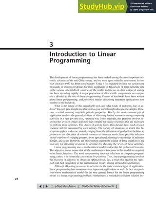
The final step is to pick out the point in this feasible region that maximizes the
value of Z ⫽ 3x1 ⫹ 5x2. To discover how to perform this step efficiently, begin by trial
and error. Try, for example, Z ⫽ 10 ⫽ 3x1 ⫹ 5x2 to see if there are in the permissible
region any values of (x1, x2) that yield a value of Z as large as 10. By drawing the line
3x1 ⫹ 5x2 ⫽ 10 (see Fig. 3.3), you can see that there are many points on this line that
lie within the region. Having gained perspective by trying this arbitrarily chosen value
of Z ⫽ 10, you should next try a larger arbitrary value of Z, say, Z ⫽ 20 ⫽ 3x1 ⫹ 5x2.
Again, Fig. 3.3 reveals that a segment of the line 3x1 ⫹ 5x2 ⫽ 20 lies within the region,
so that the maximum permissible value of Z must be at least 20.
Now notice in Fig. 3.3 that the two lines just constructed are parallel. This is no co-
incidence, since any line constructed in this way has the form Z ⫽ 3x1 ⫹ 5x2 for the cho-
sen value of Z, which implies that 5x2 ⫽ ⫺3x1 ⫹ Z or, equivalently,
x2 ⫽ ⫺ᎏ
3
5
ᎏx1 ⫹ ᎏ
1
5
ᎏZ
This last equation, called the slope-intercept form of the objective function, demonstrates
that the slope of the line is ⫺ᎏ
3
5
ᎏ (since each unit increase in x1 changes x2 by ⫺ᎏ
3
5
ᎏ), whereas
the intercept of the line with the x2 axis is ᎏ
1
5
ᎏZ (since x2 ⫽ ᎏ
1
5
ᎏZ when x1 ⫽ 0). The fact that
the slope is fixed at ⫺ᎏ
3
5
ᎏ means that all lines constructed in this way are parallel.
Again, comparing the 10 ⫽ 3x1 ⫹ 5x2 and 20 ⫽ 3x1 ⫹ 5x2 lines in Fig. 3.3, we note
that the line giving a larger value of Z (Z ⫽ 20) is farther up and away from the origin
than the other line (Z ⫽ 10). This fact also is implied by the slope-intercept form of the
objective function, which indicates that the intercept with the x1 axis (ᎏ
1
5
ᎏZ) increases when
the value chosen for Z is increased.
FIGURE 3.3
The value of (x1, x2) that
maximizes 3x1 ⫹ 5x2 is (2, 6).
2
4
6
8
x2
6 8 x1
0 10
Z ⫽ 36 ⫽ 3x1 ⫹ 5x2
Z ⫽ 20 ⫽ 3x1 ⫹ 5x2
Z ⫽ 10 ⫽ 3x1 ⫹ 5x2
2 4 x1
(2, 6)
| | | |
▲
▲

These observations imply that our trial-and-error procedure for constructing lines in Fig.
3.3 involves nothing more than drawing a family of parallel lines containing at least one point
in the feasible region and selecting the line that corresponds to the largest value of Z. Figure
3.3 shows that this line passes through the point (2, 6), indicating that the optimal solution
is x1 ⫽ 2 and x2 ⫽ 6. The equation of this line is 3x1 ⫹ 5x2 ⫽ 3(2) ⫹ 5(6) ⫽ 36 ⫽ Z, indi-
cating that the optimal value of Z is Z ⫽ 36. The point (2, 6) lies at the intersection of the
two lines 2x2 ⫽ 12 and 3x1 ⫹ 2x2 ⫽ 18, shown in Fig. 3.2, so that this point can be calcu-
lated algebraically as the simultaneous solution of these two equations.
Having seen the trial-and-error procedure for finding the optimal point (2, 6), you
now can streamline this approach for other problems. Rather than draw several parallel
lines, it is sufficient to form a single line with a ruler to establish the slope. Then move
the ruler with fixed slope through the feasible region in the direction of improving Z.
(When the objective is to minimize Z, move the ruler in the direction that decreases Z.)
Stop moving the ruler at the last instant that it still passes through a point in this region.
This point is the desired optimal solution.
This procedure often is referred to as the graphical method for linear programming. It
can be used to solve any linear programming problem with two decision variables. With con-
siderable difficulty, it is possible to extend the method to three decision variables but not more
than three. (The next chapter will focus on the simplex method for solving larger problems.)
Conclusions
The OR team used this approach to find that the optimal solution is x1 ⫽ 2, x2 ⫽ 6, with
Z ⫽ 36. This solution indicates that the Wyndor Glass Co. should produce products 1 and
2 at the rate of 2 batches per week and 6 batches per week, respectively, with a resulting
total profit of $36,000 per week. No other mix of the two products would be so prof-
itable—according to the model.
However, we emphasized in Chap. 2 that well-conducted OR studies do not simply
find one solution for the initial model formulated and then stop. All six phases described
in Chap. 2 are important, including thorough testing of the model (see Sec. 2.4) and postop-
timality analysis (see Sec. 2.3).
In full recognition of these practical realities, the OR team now is ready to evaluate
the validity of the model more critically (to be continued in Sec. 3.3) and to perform sen-
sitivity analysis on the effect of the estimates in Table 3.1 being different because of in-
accurate estimation, changes of circumstances, etc. (to be continued in Sec. 6.7).
Continuing the Learning Process with Your OR Courseware
This is the first of many points in the book where you may find it helpful to use your OR
Courseware in the CD-ROM that accompanies this book. A key part of this courseware
is a program called OR Tutor. This program includes a complete demonstration example
of the graphical method introduced in this section. Like the many other demonstration ex-
amples accompanying other sections of the book, this computer demonstration highlights
concepts that are difficult to convey on the printed page. You may refer to Appendix 1 for
documentation of the software.
When you formulate a linear programming model with more than two decision vari-
ables (so the graphical method cannot be used), the simplex method described in Chap. 4
OR
TUTOR
| | | |
▲
▲

enables you to still find an optimal solution immediately. Doing so also is helpful for
model validation, since finding a nonsensical optimal solution signals that you have made
a mistake in formulating the model.
We mentioned in Sec. 1.4 that your OR Courseware introduces you to three particu-
larly popular commercial software packages—the Excel Solver, LINGO/LINDO, and
MPL/CPLEX—for solving a variety of OR models. All three packages include the sim-
plex method for solving linear programming models. Section 3.6 describes how to use
Excel to formulate and solve linear programming models in a spreadsheet format. De-
scriptions of the other packages are provided in Sec. 3.7 (MPL and LINGO), Appendix
3.1 (LINGO), Sec. 4.8 (CPLEX and LINDO), and Appendix 4.1 (LINDO). In addition,
your OR Courseware includes a file for each of the three packages showing how it can
be used to solve each of the examples in this chapter.
3.2 THE LINEAR PROGRAMMING MODEL 31
The Wyndor Glass Co. problem is intended to illustrate a typical linear programming prob-
lem (miniature version). However, linear programming is too versatile to be completely
characterized by a single example. In this section we discuss the general characteristics
of linear programming problems, including the various legitimate forms of the mathe-
matical model for linear programming.
Let us begin with some basic terminology and notation. The first column of Table 3.2
summarizes the components of the Wyndor Glass Co. problem. The second column then
introduces more general terms for these same components that will fit many linear pro-
gramming problems. The key terms are resources and activities, where m denotes the num-
ber of different kinds of resources that can be used and n denotes the number of activi-
ties being considered. Some typical resources are money and particular kinds of machines,
equipment, vehicles, and personnel. Examples of activities include investing in particular
projects, advertising in particular media, and shipping goods from a particular source to
a particular destination. In any application of linear programming, all the activities may
be of one general kind (such as any one of these three examples), and then the individ-
ual activities would be particular alternatives within this general category.
As described in the introduction to this chapter, the most common type of applica-
tion of linear programming involves allocating resources to activities. The amount avail-
able of each resource is limited, so a careful allocation of resources to activities must be
made. Determining this allocation involves choosing the levels of the activities that achieve
the best possible value of the overall measure of performance.
3.2 THE LINEAR PROGRAMMING MODEL
TABLE 3.2 Common terminology for linear programming
Prototype Example General Problem
Production capacities of plants Resources
3 plants m resources
Production of products Activities
2 products n activities
Production rate of product j, xj Level of activity j, xj
Profit Z Overall measure of performance Z
| | | |
▲
▲

Certain symbols are commonly used to denote the various components of a linear
programming model. These symbols are listed below, along with their interpretation for
the general problem of allocating resources to activities.
Z ⫽ value of overall measure of performance.
xj ⫽ level of activity j (for j ⫽ 1, 2, . . . , n).
cj ⫽ increase in Z that would result from each unit increase in level of activity j.
bi ⫽ amount of resource i that is available for allocation to activities (for i ⫽
1, 2, . . . , m).
aij ⫽ amount of resource i consumed by each unit of activity j.
The model poses the problem in terms of making decisions about the levels of the activ-
ities, so x1, x2, . . . , xn are called the decision variables. As summarized in Table 3.3, the
values of cj, bi, and aij (for i ⫽ 1, 2, . . . , m and j ⫽ 1, 2, . . . , n) are the input constants
for the model. The cj, bi, and aij are also referred to as the parameters of the model.
Notice the correspondence between Table 3.3 and Table 3.1.
A Standard Form of the Model
Proceeding as for the Wyndor Glass Co. problem, we can now formulate the mathemati-
cal model for this general problem of allocating resources to activities. In particular, this
model is to select the values for x1, x2, . . . , xn so as to
Maximize Z ⫽ c1x1 ⫹ c2x2 ⫹ ⭈⭈⭈ ⫹ cnxn,
subject to the restrictions
a11x1 ⫹ a12x2 ⫹ ⭈⭈⭈ ⫹ a1nxn ⱕ b1
a21x1 ⫹ a22x2 ⫹ ⭈⭈⭈ ⫹ a2nxn ⱕ b2
⯗
am1x1 ⫹ am2x2 ⫹ ⭈⭈⭈ ⫹ amnxn ⱕ bm,
TABLE 3.3 Data needed for a linear programming model involving the allocation
of resources to activities
Resource Usage per Unit of Activity
Activity
Amount of
Resource 1 2 . . . n Resource Available
1 a11 a12 . . . a1n b1
2 a21 a22 . . . a2n b2
. .
. . . . . . . . . . . . . .
. .
m am1 am2 . . . amn bm
Contribution to Z per c1 c2 . . . cn
unit of activity
| | | |
▲
▲

and
x1 ⱖ 0, x2 ⱖ 0, . . . , xn ⱖ 0.
We call this our standard form1
for the linear programming problem. Any situation whose
mathematical formulation fits this model is a linear programming problem.
Notice that the model for the Wyndor Glass Co. problem fits our standard form, with
m ⫽ 3 and n ⫽ 2.
Common terminology for the linear programming model can now be summarized.
The function being maximized, c1x1 ⫹ c2x2 ⫹ ⭈⭈⭈ ⫹ cnxn, is called the objective func-
tion. The restrictions normally are referred to as constraints. The first m constraints (those
with a function of all the variables ai1x1 ⫹ ai2x2 ⫹ ⭈⭈⭈ ⫹ ainxn on the left-hand side) are
sometimes called functional constraints (or structural constraints). Similarly, the xj ⱖ 0
restrictions are called nonnegativity constraints (or nonnegativity conditions).
Other Forms
We now hasten to add that the preceding model does not actually fit the natural form of
some linear programming problems. The other legitimate forms are the following:
1. Minimizing rather than maximizing the objective function:
Minimize Z ⫽ c1x1 ⫹ c2x2 ⫹ ⭈⭈⭈ ⫹ cnxn.
2. Some functional constraints with a greater-than-or-equal-to inequality:
ai1x1 ⫹ ai2x2 ⫹ ⭈⭈⭈ ⫹ ainxn ⱖ bi for some values of i.
3. Some functional constraints in equation form:
ai1x1 ⫹ ai2x2 ⫹ ⭈⭈⭈ ⫹ ainxn ⫽ bi for some values of i.
4. Deleting the nonnegativity constraints for some decision variables:
xj unrestricted in sign for some values of j.
Any problem that mixes some of or all these forms with the remaining parts of the pre-
ceding model is still a linear programming problem. Our interpretation of the words al-
locating limited resources among competing activities may no longer apply very well, if
at all; but regardless of the interpretation or context, all that is required is that the math-
ematical statement of the problem fit the allowable forms.
Terminology for Solutions of the Model
You may be used to having the term solution mean the final answer to a problem, but the
convention in linear programming (and its extensions) is quite different. Here, any spec-
ification of values for the decision variables (x1, x2, . . . , xn) is called a solution, regard-
less of whether it is a desirable or even an allowable choice. Different types of solutions
are then identified by using an appropriate adjective.
1
This is called our standard form rather than the standard form because some textbooks adopt other forms.
| | | |
▲
▲

A feasible solution is a solution for which all the constraints are satisfied.
An infeasible solution is a solution for which at least one constraint is violated.
In the example, the points (2, 3) and (4, 1) in Fig. 3.2 are feasible solutions, while the
points (⫺1, 3) and (4, 4) are infeasible solutions.
The feasible region is the collection of all feasible solutions.
The feasible region in the example is the entire shaded area in Fig. 3.2.
It is possible for a problem to have no feasible solutions. This would have happened
in the example if the new products had been required to return a net profit of at least
$50,000 per week to justify discontinuing part of the current product line. The corre-
sponding constraint, 3x1 ⫹ 5x2 ⱖ 50, would eliminate the entire feasible region, so no mix
of new products would be superior to the status quo. This case is illustrated in Fig. 3.4.
Given that there are feasible solutions, the goal of linear programming is to find a
best feasible solution, as measured by the value of the objective function in the model.
An optimal solution is a feasible solution that has the most favorable value of
the objective function.
The most favorable value is the largest value if the objective function is to be maximized,
whereas it is the smallest value if the objective function is to be minimized.
Most problems will have just one optimal solution. However, it is possible to have more
than one. This would occur in the example if the profit per batch produced of product 2 were
changed to $2,000. This changes the objective function to Z ⫽ 3x1 ⫹ 2x2, so that all the points
2
4
6
8
x2
2 4 6 8 x1
0 10
10
3x1 ⫹ 5x2 ⱖ 50
2x2 ⱕ 12
3x1 ⫹ 2x2 ⱕ 18
x1 ⱖ 0
x2 ⱖ 0
x1 ⱕ 4
subject to x1 ⱕ 4
ⱕ 12
ⱕ 18
ⱖ 50
2x2
2x2
5x2
3x1 ⫹
3x1 ⫹
x1 ⱖ 0, x2 ⱖ 0
and
FIGURE 3.4
The Wyndor Glass Co.
problem would have no
feasible solutions if the
constraint 3x1 ⫹ 5x2 ⱖ 50
were added to the problem.
| | | |
▲
▲

on the line segment connecting (2, 6) and (4, 3) would be optimal. This case is illustrated in
Fig. 3.5. As in this case, any problem having multiple optimal solutions will have an infi-
nite number of them, each with the same optimal value of the objective function.
Another possibility is that a problem has no optimal solutions. This occurs only if
(1) it has no feasible solutions or (2) the constraints do not prevent improving the value
of the objective function (Z) indefinitely in the favorable direction (positive or negative).
The latter case is referred to as having an unbounded Z. To illustrate, this case would re-
sult if the last two functional constraints were mistakenly deleted in the example, as il-
lustrated in Fig. 3.6.
We next introduce a special type of feasible solution that plays the key role when the
simplex method searches for an optimal solution.
A corner-point feasible (CPF) solution is a solution that lies at a corner of the
feasible region.
Figure 3.7 highlights the five CPF solutions for the example.
Sections 4.1 and 5.1 will delve into the various useful properties of CPF solutions for
problems of any size, including the following relationship with optimal solutions.
Relationship between optimal solutions and CPF solutions: Consider any linear pro-
gramming problem with feasible solutions and a bounded feasible region. The problem
must possess CPF solutions and at least one optimal solution. Furthermore, the best CPF
solution must be an optimal solution. Thus, if a problem has exactly one optimal solution,
it must be a CPF solution. If the problem has multiple optimal solutions, at least two must
be CPF solutions.
FIGURE 3.5
problem would have multiple
optimal solutions if the
objective function were
changed to Z ⫽ 3x1 ⫹ 2x2.
| | | |
▲
▲

2
4
6
8
x2
2 4 6 8 x1
0 10
subject to
and
x1 ⱕ 4
x1 ⱖ 0, x2 ⱖ 0
10
(4, 2), Z ⫽ 22
(4, 4), Z ⫽ 32
(4, 6), Z ⫽ 42
(4, 8), Z ⫽ 52
(4, 10), Z ⫽ 62
(4, ⬁), Z ⫽ ⬁
Feasible
region
FIGURE 3.6
problem would have no
optimal solutions if the only
functional constraint were
x1 ⱕ 4, because x2 then
could be increased
indefinitely in the feasible
region without ever reaching
the maximum value of
Z ⫽ 3x1 ⫹ 5x2.
All the assumptions of linear programming actually are implicit in the model formulation
given in Sec. 3.2. However, it is good to highlight these assumptions so you can more
easily evaluate how well linear programming applies to any given problem. Furthermore,
we still need to see why the OR team for the Wyndor Glass Co. concluded that a linear
programming formulation provided a satisfactory representation of the problem.
Proportionality
Proportionality is an assumption about both the objective function and the functional con-
straints, as summarized below.
Proportionality assumption: The contribution of each activity to the value of
the objective function Z is proportional to the level of the activity xj, as repre-
sented by the cjxj term in the objective function. Similarly, the contribution of
each activity to the left-hand side of each functional constraint is proportional
to the level of the activity xj, as represented by the aijxj term in the constraint.
3.3 ASSUMPTIONS OF LINEAR PROGRAMMING
The example has exactly one optimal solution, (x1, x2) ⫽ (2, 6), which is a CPF so-
lution. (Think about how the graphical method leads to the one optimal solution being a
CPF solution.) When the example is modified to yield multiple optimal solutions, as shown
in Fig. 3.5, two of these optimal solutions—(2, 6) and (4, 3)—are CPF solutions.
| | | |
▲
▲

3.3 ASSUMPTIONS OF LINEAR PROGRAMMING 37
(0, 6) (2, 6)
x2
(4, 0)
(4, 3)
x1
Feasible
region
(0, 0)
FIGURE 3.7
The five dots are the five CPF
solutions for the Wyndor
Glass Co. problem.
1
When the function includes any cross-product terms, proportionality should be interpreted to mean that changes
in the function value are proportional to changes in each variable (xj) individually, given any fixed values for
all the other variables. Therefore, a cross-product term satisfies proportionality as long as each variable in the
term has an exponent of 1. (However, any cross-product term violates the additivity assumption, discussed next.)
TABLE 3.4 Examples of satisfying or violating proportionality
Profit from Product 1 ($000 per Week)
Proportionality Violated
Proportionality
x1 Satisfied Case 1 Case 2 Case 3
0 0 0 0 0
1 3 2 3 3
2 6 5 7 5
3 9 8 12 6
4 12 11 18 6
Consequently, this assumption rules out any exponent other than 1 for any vari-
able in any term of any function (whether the objective function or the function
on the left-hand side of a functional constraint) in a linear programming model.1
To illustrate this assumption, consider the first term (3x1) in the objective function
(Z ⫽ 3x1 ⫹ 5x2) for the Wyndor Glass Co. problem. This term represents the profit gen-
erated per week (in thousands of dollars) by producing product 1 at the rate of x1 batches
per week. The proportionality satisfied column of Table 3.4 shows the case that was as-
sumed in Sec. 3.1, namely, that this profit is indeed proportional to x1 so that 3x1 is the
appropriate term for the objective function. By contrast, the next three columns show dif-
ferent hypothetical cases where the proportionality assumption would be violated.
Refer first to the Case 1 column in Table 3.4. This case would arise if there were
start-up costs associated with initiating the production of product 1. For example, there
| | | |
▲
▲

might be costs involved with setting up the production facilities. There might also be costs
associated with arranging the distribution of the new product. Because these are one-time
costs, they would need to be amortized on a per-week basis to be commensurable with Z
(profit in thousands of dollars per week). Suppose that this amortization were done and
that the total start-up cost amounted to reducing Z by 1, but that the profit without con-
sidering the start-up cost would be 3x1. This would mean that the contribution from prod-
uct 1 to Z should be 3x1 ⫺ 1 for x1 ⬎ 0, whereas the contribution would be 3x1 ⫽ 0 when
x1 ⫽ 0 (no start-up cost). This profit function,1
which is given by the solid curve in Fig.
3.8, certainly is not proportional to x1.
At first glance, it might appear that Case 2 in Table 3.4 is quite similar to Case 1.
However, Case 2 actually arises in a very different way. There no longer is a start-up cost,
and the profit from the first unit of product 1 per week is indeed 3, as originally assumed.
However, there now is an increasing marginal return; i.e., the slope of the profit function
for product 1 (see the solid curve in Fig. 3.9) keeps increasing as x1 is increased. This vi-
olation of proportionality might occur because of economies of scale that can sometimes
be achieved at higher levels of production, e.g., through the use of more efficient high-
volume machinery, longer production runs, quantity discounts for large purchases of raw
materials, and the learning-curve effect whereby workers become more efficient as they
gain experience with a particular mode of production. As the incremental cost goes down,
the incremental profit will go up (assuming constant marginal revenue).
x1
0
1 2 3 4
Start-up cost
⫺3
3
6
9
Satisfies
proportionality
assumption
Violates
proportionality
assumption
12
Contribution
of x1 to Z
FIGURE 3.8
The solid curve violates the
proportionality assumption
because of the start-up cost
that is incurred when x1 is
increased from 0. The values
at the dots are given by the
Case 1 column of Table 3.4.
1
If the contribution from product 1 to Z were 3x1 ⫺ 1 for all x1 ⱖ 0, including x1 ⫽ 0, then the fixed constant,
⫺1, could be deleted from the objective function without changing the optimal solution and proportionality
would be restored. However, this “fix” does not work here because the ⫺1 constant does not apply when
x1 ⫽ 0.
| | | |
▲
▲

Referring again to Table 3.4, the reverse of Case 2 is Case 3, where there is a decreas-
ing marginal return. In this case, the slope of the profit function for product 1 (given by the
solid curve in Fig. 3.10) keeps decreasing as x1 is increased. This violation of proportional-
ity might occur because the marketing costs need to go up more than proportionally to attain
increases in the level of sales. For example, it might be possible to sell product 1 at the rate
of 1 per week (x1 ⫽ 1) with no advertising, whereas attaining sales to sustain a production
rate of x1 ⫽ 2 might require a moderate amount of advertising, x1 ⫽ 3 might necessitate an
extensive advertising campaign, and x1 ⫽ 4 might require also lowering the price.
All three cases are hypothetical examples of ways in which the proportionality as-
sumption could be violated. What is the actual situation? The actual profit from produc-
0 1 2 3 4 x1
3
6
9
12
15
18
Contribution
of x1 to Z
Violates
proportionality
assumption
Satisfies
proportionality
assumption
FIGURE 3.9
because its slope (the
marginal return from
product 1) keeps increasing
as x1 is increased. The values
Case 2 column of Table 3.4.
0 1 2 3 4 x1
3
6
9
12
Contribution
of x1 to Z
Violates
proportionality
assumption
Satisfies
proportionality
assumption
FIGURE 3.10
because its slope (the
marginal return from
product 1) keeps decreasing
as x1 is increased. The values
Case 3 column in Table 3.4.
| | | |
▲
▲

ing product 1 (or any other product) is derived from the sales revenue minus various di-
rect and indirect costs. Inevitably, some of these cost components are not strictly propor-
tional to the production rate, perhaps for one of the reasons illustrated above. However,
the real question is whether, after all the components of profit have been accumulated,
proportionality is a reasonable approximation for practical modeling purposes. For the
Wyndor Glass Co. problem, the OR team checked both the objective function and the
functional constraints. The conclusion was that proportionality could indeed be assumed
without serious distortion.
For other problems, what happens when the proportionality assumption does not hold
even as a reasonable approximation? In most cases, this means you must use nonlinear
programming instead (presented in Chap. 13). However, we do point out in Sec. 13.8 that
a certain important kind of nonproportionality can still be handled by linear programming
by reformulating the problem appropriately. Furthermore, if the assumption is violated
only because of start-up costs, there is an extension of linear programming (mixed inte-
ger programming) that can be used, as discussed in Sec. 12.3 (the fixed-charge problem).
Additivity
Although the proportionality assumption rules out exponents other than 1, it does not pro-
hibit cross-product terms (terms involving the product of two or more variables). The ad-
ditivity assumption does rule out this latter possibility, as summarized below.
Additivity assumption: Every function in a linear programming model (whether
the objective function or the function on the left-hand side of a functional con-
straint) is the sum of the individual contributions of the respective activities.
To make this definition more concrete and clarify why we need to worry about this
assumption, let us look at some examples. Table 3.5 shows some possible cases for the ob-
jective function for the Wyndor Glass Co. problem. In each case, the individual contribu-
tions from the products are just as assumed in Sec. 3.1, namely, 3x1 for product 1 and 5x2
for product 2. The difference lies in the last row, which gives the function value for Z when
the two products are produced jointly. The additivity satisfied column shows the case where
this function value is obtained simply by adding the first two rows (3 ⫹ 5 ⫽ 8), so that
Z ⫽ 3x1 ⫹ 5x2 as previously assumed. By contrast, the next two columns show hypothet-
ical cases where the additivity assumption would be violated (but not the proportionality
assumption).
TABLE 3.5 Examples of satisfying or violating additivity for the objective function
Value of Z
Additivity Violated
(x1, x2) Additivity Satisfied Case 1 Case 2
(1, 0) 3 3 3
(0, 1) 5 5 5
(1, 1) 8 9 7
| | | |
▲
▲

Referring to the Case 1 column of Table 3.5, this case corresponds to an objective
function of Z ⫽ 3x1 ⫹ 5x2 ⫹ x1x2, so that Z ⫽ 3 ⫹ 5 ⫹ 1 ⫽ 9 for (x1, x2) ⫽ (1, 1), thereby
violating the additivity assumption that Z ⫽ 3 ⫹ 5. (The proportionality assumption still
is satisfied since after the value of one variable is fixed, the increment in Z from the other
variable is proportional to the value of that variable.) This case would arise if the two
products were complementary in some way that increases profit. For example, suppose
that a major advertising campaign would be required to market either new product pro-
duced by itself, but that the same single campaign can effectively promote both products
if the decision is made to produce both. Because a major cost is saved for the second
product, their joint profit is somewhat more than the sum of their individual profits when
each is produced by itself.
Case 2 in Table 3.5 also violates the additivity assumption because of the extra term
in the corresponding objective function, Z ⫽ 3x1 ⫹ 5x2 ⫺ x1x2, so that Z ⫽ 3 ⫹ 5 ⫺ 1 ⫽ 7
for (x1, x2) ⫽ (1, 1). As the reverse of the first case, Case 2 would arise if the two prod-
ucts were competitive in some way that decreased their joint profit. For example, suppose
that both products need to use the same machinery and equipment. If either product were
produced by itself, this machinery and equipment would be dedicated to this one use.
However, producing both products would require switching the production processes back
and forth, with substantial time and cost involved in temporarily shutting down the pro-
duction of one product and setting up for the other. Because of this major extra cost, their
joint profit is somewhat less than the sum of their individual profits when each is pro-
duced by itself.
The same kinds of interaction between activities can affect the additivity of the con-
straint functions. For example, consider the third functional constraint of the Wyndor Glass
Co. problem: 3x1 ⫹ 2x2 ⱕ 18. (This is the only constraint involving both products.) This
constraint concerns the production capacity of Plant 3, where 18 hours of production time
per week is available for the two new products, and the function on the left-hand side
(3x1 ⫹ 2x2) represents the number of hours of production time per week that would be
used by these products. The additivity satisfied column of Table 3.6 shows this case as is,
whereas the next two columns display cases where the function has an extra cross-
product term that violates additivity. For all three columns, the individual contributions
from the products toward using the capacity of Plant 3 are just as assumed previously,
namely, 3x1 for product 1 and 2x2 for product 2, or 3(2) ⫽ 6 for x1 ⫽ 2 and 2(3) ⫽ 6 for
TABLE 3.6 Examples of satisfying or violating additivity
for a functional constraint
Amount of Resource Used
Additivity Violated
(x1, x2) Additivity Satisfied Case 3 Case 4
(2, 0) 6 6 6
(0, 3) 6 6 6
(2, 3) 12 15 10.8
| | | |
▲
▲

x2 ⫽ 3. As was true for Table 3.5, the difference lies in the last row, which now gives the
total function value for production time used when the two products are produced jointly.
For Case 3 (see Table 3.6), the production time used by the two products is given by
the function 3x1 ⫹ 2x2 ⫹ 0.5x1x2, so the total function value is 6 ⫹ 6 ⫹ 3 ⫽ 15 when
(x1, x2) ⫽ (2, 3), which violates the additivity assumption that the value is just 6 ⫹ 6 ⫽ 12.
This case can arise in exactly the same way as described for Case 2 in Table 3.5; namely,
extra time is wasted switching the production processes back and forth between the two
products. The extra cross-product term (0.5x1x2) would give the production time wasted
in this way. (Note that wasting time switching between products leads to a positive cross-
product term here, where the total function is measuring production time used, whereas
it led to a negative cross-product term for Case 2 because the total function there mea-
sures profit.)
For Case 4 in Table 3.6, the function for production time used is 3x1 ⫹ 2x2 ⫺ 0.1x1
2
x2,
so the function value for (x1, x2) ⫽ (2, 3) is 6 ⫹ 6 ⫺ 1.2 ⫽ 10.8. This case could arise in
the following way. As in Case 3, suppose that the two products require the same type of
machinery and equipment. But suppose now that the time required to switch from one
product to the other would be relatively small. Because each product goes through a se-
quence of production operations, individual production facilities normally dedicated to
that product would incur occasional idle periods. During these otherwise idle periods,
these facilities can be used by the other product. Consequently, the total production time
used (including idle periods) when the two products are produced jointly would be less
than the sum of the production times used by the individual products when each is pro-
duced by itself.
After analyzing the possible kinds of interaction between the two products illustrated
by these four cases, the OR team concluded that none played a major role in the actual
Wyndor Glass Co. problem. Therefore, the additivity assumption was adopted as a rea-
sonable approximation.
For other problems, if additivity is not a reasonable assumption, so that some of or
all the mathematical functions of the model need to be nonlinear (because of the cross-
product terms), you definitely enter the realm of nonlinear programming (Chap. 13).
Divisibility
Our next assumption concerns the values allowed for the decision variables.
Divisibility assumption: Decision variables in a linear programming model are
allowed to have any values, including noninteger values, that satisfy the func-
tional and nonnegativity constraints. Thus, these variables are not restricted to
just integer values. Since each decision variable represents the level of some ac-
tivity, it is being assumed that the activities can be run at fractional levels.
For the Wyndor Glass Co. problem, the decision variables represent production rates
(the number of batches of a product produced per week). Since these production rates can
have any fractional values within the feasible region, the divisibility assumption does hold.
In certain situations, the divisibility assumption does not hold because some of or all
the decision variables must be restricted to integer values. Mathematical models with this
restriction are called integer programming models, and they are discussed in Chap. 12.
| | | |
▲
▲

Certainty
Our last assumption concerns the parameters of the model, namely, the coefficients in the
objective function cj, the coefficients in the functional constraints aij, and the right-hand
sides of the functional constraints bi.
Certainty assumption: The value assigned to each parameter of a linear pro-
gramming model is assumed to be a known constant.
In real applications, the certainty assumption is seldom satisfied precisely. Linear pro-
gramming models usually are formulated to select some future course of action. There-
fore, the parameter values used would be based on a prediction of future conditions, which
inevitably introduces some degree of uncertainty.
For this reason it is usually important to conduct sensitivity analysis after a solution
is found that is optimal under the assumed parameter values. As discussed in Sec. 2.3,
one purpose is to identify the sensitive parameters (those whose value cannot be changed
without changing the optimal solution), since any later change in the value of a sensitive
parameter immediately signals a need to change the solution being used.
Sensitivity analysis plays an important role in the analysis of the Wyndor Glass Co.
problem, as you will see in Sec. 6.7. However, it is necessary to acquire some more back-
ground before we finish that story.
Occasionally, the degree of uncertainty in the parameters is too great to be amenable
to sensitivity analysis. In this case, it is necessary to treat the parameters explicitly as ran-
dom variables. Formulations of this kind have been developed, as discussed in Secs. 23.6
and 23.7 on the book’s web site, w
www.mhhe.com/hillier.
The Assumptions in Perspective
We emphasized in Sec. 2.2 that a mathematical model is intended to be only an idealized
representation of the real problem. Approximations and simplifying assumptions gener-
ally are required in order for the model to be tractable. Adding too much detail and pre-
cision can make the model too unwieldy for useful analysis of the problem. All that is re-
ally needed is that there be a reasonably high correlation between the prediction of the
model and what would actually happen in the real problem.
This advice certainly is applicable to linear programming. It is very common in real
applications of linear programming that almost none of the four assumptions hold com-
pletely. Except perhaps for the divisibility assumption, minor disparities are to be expected.
This is especially true for the certainty assumption, so sensitivity analysis normally is a
must to compensate for the violation of this assumption.
However, it is important for the OR team to examine the four assumptions for the
problem under study and to analyze just how large the disparities are. If any of the as-
sumptions are violated in a major way, then a number of useful alternative models are
available, as presented in later chapters of the book. A disadvantage of these other mod-
els is that the algorithms available for solving them are not nearly as powerful as those
for linear programming, but this gap has been closing in some cases. For some applica-
tions, the powerful linear programming approach is used for the initial analysis, and then
a more complicated model is used to refine this analysis.
| | | |
▲
▲

As you work through the examples in the next section, you will find it good practice
to analyze how well each of the four assumptions of linear programming applies.
The Wyndor Glass Co. problem is a prototype example of linear programming in several
respects: It involves allocating limited resources among competing activities, its model
fits our standard form, and its context is the traditional one of improved business plan-
ning. However, the applicability of linear programming is much wider. In this section we
begin broadening our horizons. As you study the following examples, note that it is their
underlying mathematical model rather than their context that characterizes them as linear
programming problems. Then give some thought to how the same mathematical model
could arise in many other contexts by merely changing the names of the activities and so
forth.
These examples are scaled-down versions of actual applications (including two that
are included in the case studies presented in the next section).
Design of Radiation Therapy
MARY has just been diagnosed as having a cancer at a fairly advanced stage. Specifi-
cally, she has a large malignant tumor in the bladder area (a “whole bladder lesion”).
Mary is to receive the most advanced medical care available to give her every possi-
ble chance for survival. This care will include extensive radiation therapy.
Radiation therapy involves using an external beam treatment machine to pass ioniz-
ing radiation through the patient’s body, damaging both cancerous and healthy tissues.
Normally, several beams are precisely administered from different angles in a two-
dimensional plane. Due to attenuation, each beam delivers more radiation to the tissue
near the entry point than to the tissue near the exit point. Scatter also causes some deliv-
ery of radiation to tissue outside the direct path of the beam. Because tumor cells are typ-
ically microscopically interspersed among healthy cells, the radiation dosage throughout
the tumor region must be large enough to kill the malignant cells, which are slightly more
radiosensitive, yet small enough to spare the healthy cells. At the same time, the aggre-
gate dose to critical tissues must not exceed established tolerance levels, in order to pre-
vent complications that can be more serious than the disease itself. For the same reason,
the total dose to the entire healthy anatomy must be minimized.
Because of the need to carefully balance all these factors, the design of radiation ther-
apy is a very delicate process. The goal of the design is to select the combination of beams
to be used, and the intensity of each one, to generate the best possible dose distribution.
(The dose strength at any point in the body is measured in units called kilorads.) Once
the treatment design has been developed, it is administered in many installments, spread
over several weeks.
In Mary’s case, the size and location of her tumor make the design of her treatment
an even more delicate process than usual. Figure 3.11 shows a diagram of a cross section
of the tumor viewed from above, as well as nearby critical tissues to avoid. These tissues
include critical organs (e.g., the rectum) as well as bony structures (e.g., the femurs and
pelvis) that will attenuate the radiation. Also shown are the entry point and direction for
the only two beams that can be used with any modicum of safety in this case. (Actually,
3.4 ADDITIONAL EXAMPLES
Beam 2
Beam 1
1
2
3 3
1. Bladder and
tumor
2. Rectum, coccyx,
etc.
3. Femur, part of
pelvis, etc.
FIGURE 3.11
Cross section of Mary’s
tumor (viewed from above),
nearby critical tissues, and
the radiation beams being
used.
MPL
| | | |
▲
▲

3 Introduction To Linear Programming

Recommended

Recommended

More Related Content

Similar to 3 Introduction To Linear Programming

Similar to 3 Introduction To Linear Programming (20)

More from Dawn Cook

More from Dawn Cook (20)

Recently uploaded

Recently uploaded (20)

3 Introduction To Linear Programming