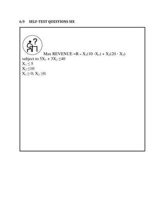
This document outlines a course on mathematics for economists. It introduces linear programming techniques for solving constrained and unconstrained optimization problems. The course objectives are to learn how to formulate and solve linear programming problems using graphical and simplex methods, test for linear dependence and convexity/concavity, and solve nonlinear programming problems, differential equations, and difference equations as applied to economics. Sample problems are provided to demonstrate how to formulate linear programming problems in the standard way, specifying the objective, decision variables, constraints, and developing the objective function.


![Max = [ … ] ⌈ ⌉
.
⌊ ⌋ ⌈ ⌉ ⌈ ⌉
, …
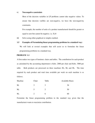
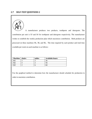
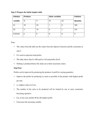
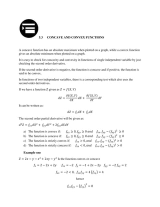
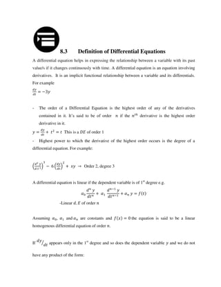
RULES OF TRANSFORMATION
The direction of optimization changes i.e maximization becomes minimization and vice versa.
e.g. min Q
The row vector of coefficient of the objective function in the primal problem is
transposed into a column vector of constants in the dual.
The column vector of constants in the constants in the primal problem is transposed
into a row vector of coefficients in the objective function of the dual.
The matrix of coefficients in the constraint equation of the primal problem is
transposed into a matrix of coefficients in the matrix of the dual problem.
The inequality sign in the primal problem is reversed, i.e. in a primal maximization
problem becomes in the dual problem.
Note. 1. The non-negativity constraints remain unchanged.
2. The decision variables will change say from Xi to Zj.](https://image.slidesharecdn.com/ees300module-181201121150/85/Ees-300-40-320.jpg)
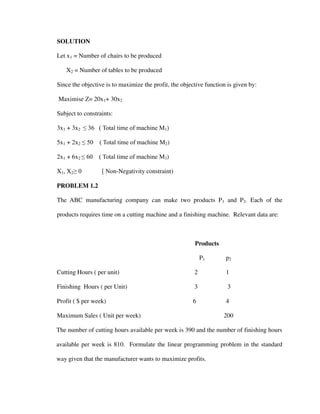
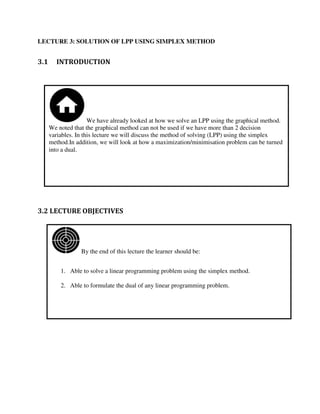
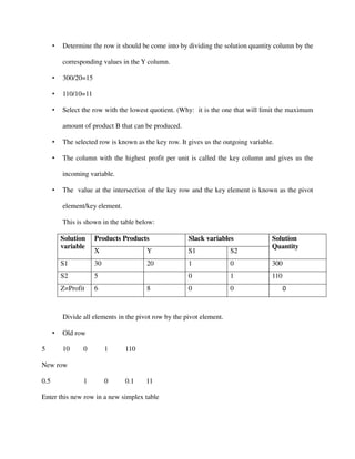
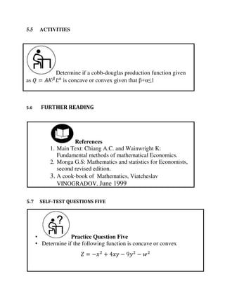
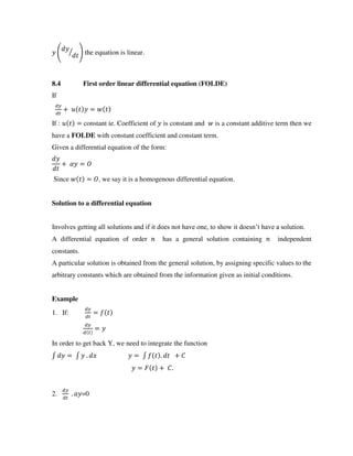
![The dual problem therefore becomes, in matrix form:
= [ … ] ⌈ ⌉
.
⌊ ⌋ ⌈ ⌉ ⌈ ⌉
, …
= + +
.
+ +
+ +
+ +
, …
Example
Let the primal problem be
� = +
.
+
+](https://image.slidesharecdn.com/ees300module-181201121150/85/Ees-300-41-320.jpg)
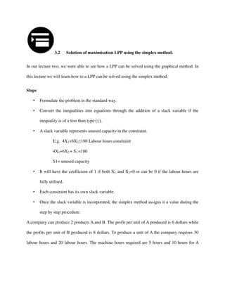
![+
Rewriting into matrix
� = [ ]
.
[ ] [ ] [ ]
The dual will be,
= [ ] [ ]
.
[ ] [ ] [ ]
In the linear form,
min = + +
.
+ +](https://image.slidesharecdn.com/ees300module-181201121150/85/Ees-300-42-320.jpg)
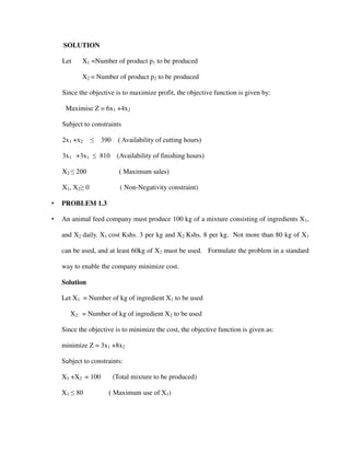
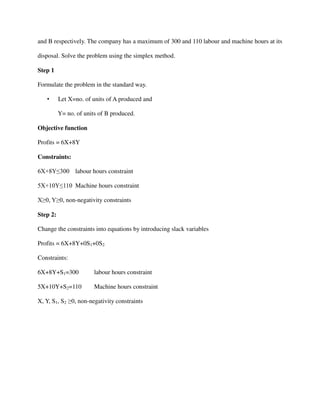
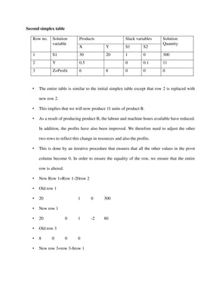
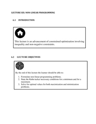
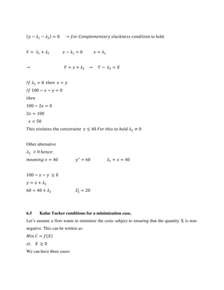
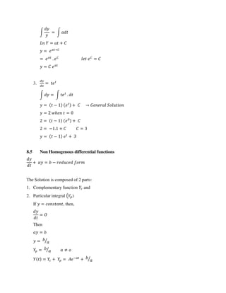
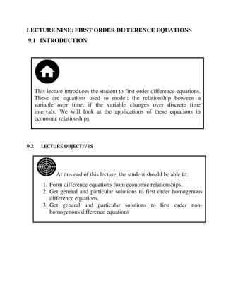
![4.3 Jacobian Determinant
The Jacobian matrix can help to test whether there exists functional linear dependence in a set of
functions in variables. It is a matrix of the first order partial derivatives. If the functions are
linearly dependent, the determinant of the Jacobian matrix is 0.
E.g. = +
= + +
�
�
=
�
�⁄ =
�
�
= +
�
�
= +
=
[
�
�
�
�
�
� ]
= |
+ +
| =
The functions are linearly dependent.
Example 2
= +
= +](https://image.slidesharecdn.com/ees300module-181201121150/85/Ees-300-46-320.jpg)
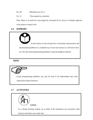
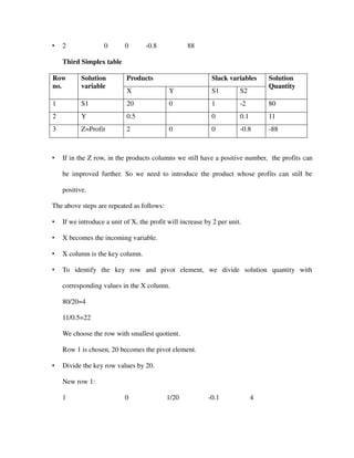
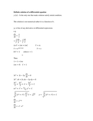
![= [ ]
| | = | |=− unless X2
Is zero, the determinant is not zero, hence the 2 functions are functionally independent.
If we have several functions,
= | | = |
′ ′
… ′
|
=
=
A Jacobian | |is identically zero for all values of , … , if the n functions are functionally
dependant.
4.4 Solution of simultaneous equations using the Gaussian method
Gaussian method involves solving for simultaneous equations using matrix algebra by getting the
lower echelon matrix for the matrix of coefficients.
If we have a matrix, given as:
+ + =
+ + =
+ + =
We can get the values of X, Y and Z by rewriting the functions in matrix form such that:
[ ] [ ] = [ ]
The lower echelon matrix for matrix of coefficients is given as:
[ ]
This is done through a step by step iteration procedure.
Let us use a practical example.](https://image.slidesharecdn.com/ees300module-181201121150/85/Ees-300-47-320.jpg)
![+ − =
+ + =
− − = −
If we rewrite the equations in matrix form, we get:
−
− −
[ ] = [
−
]
As we do the iterations, we need to maintain the row equality. This will be done by some row
operations, similar to those we used when we were looking at the simplex method in LPP. We
will only affect the matrix of the coefficients and the constants matrix. We can join them
together into one augmented matrix as we undertake the step by step procedure.
−
− −
|
−
We want to make the first element in the first row to be 1. This can be accomplished by dividing
the entire row 1 by 2. This gives us:
−
− −
|
−
The elements 2 and 3 in column 1 Row 2 and 3 respectively will be turned into 0 using the
following row procedure:
= −
= −
This gives us the following matrix:
−
−
−
| −
−
We then change the − in the second row , second column into by dividing the entire row by
− . This gives us the following matrix.
−
−
−
|
−](https://image.slidesharecdn.com/ees300module-181201121150/85/Ees-300-48-320.jpg)
![We change the value -21 in the second column into a 0 by the following procedure:
= − −
It will give us:
−
−
−
|
−
The next step involves changing the element in 3rd
row, 3rd
column into a 1. This can be done by
dividing the entire row 3 by − giving us the following matrix
−
− |
If we bring back our variables, X, Y and Z we have the following matrices:
[
−
− ] [ ] = [ ⁄ ]
+ − =
− =
=
If we replace Z=3 in the second equation, it will give us the following
− = − = → = + = =
= =
By replacing the values of Y and Z in the first equation, we get:
+ − =
= − =](https://image.slidesharecdn.com/ees300module-181201121150/85/Ees-300-49-320.jpg)
![= = =
These will be the values that will satisfy the three equations.
4.5 Gauss Jordan Elimination Method
This method is just an extension of the Gaussian method. It involves ensuring that the matrix of
coefficients is turned into an identity matrix.
Using our previous example, the matrix [
−
− ] will be changed to an identity matrix
through the same row procedures.
We will start by changing the elements − and − / in the 3rd
column, 1st
and 2nd
row
respectively into 0 using the 3rd
row. This will be done by the following process:
= − −
= − −
[ ] [ ] = [ ]
Next step involves changing the 6 in row 1 column 2 into a 0. This will be done by using row 2.
= −
It will give us:
[ ] [ ] = [ ]
We can then rewrite our matrix into equations and we will have:
=
=
=](https://image.slidesharecdn.com/ees300module-181201121150/85/Ees-300-50-320.jpg)
![Example 2
After using the Gaussian method to solve for three simultaneous equations, the following three
equations were obtained:
Determine the values of , , using the Gauss Jordan elimination method.
− . − . =
− . =
=
[
− . − .
− . ] [ ] = [ ]
Work from the last column to eliminate the coefficients of in the other rows
i.e.
= + .
= + .
− .
|
Finally change − . into a 0 by using the second row. This will be done through the following
operation:
= + .
|
= = =](https://image.slidesharecdn.com/ees300module-181201121150/85/Ees-300-51-320.jpg)
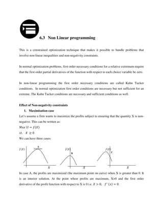
![The function Z is concave but not strictly so.
Determinantal test for sign definiteness
The matrix of second order partial derivatives: H= [ ] is called a hessian matrix.
A function Z is positive definite if the first and second principal leading minors of matrix H are
positive.
i.e. |H | = |fxx| >
|H |= | | >0 If we get the determinant, it will be given as: − >0
A function Z is negative definite if the first leading minor is negative while the second principal
leading minors of matrix H are positive.
i.e. |H | = |fxx| <
|H |= | | >0
Example Two
Determine if the following function is positive definite or negative definite using the Hessian
determinants.
= − +
= [ ]
|H | = >
|H |= | | = − = >
Since the determinants of both H1 and H2 are greater than 0, we say the function is positive
definite and by extension the function is convex.
The determinantal test can be extended to the case of more than 2 independent variables.
= , ,
= [ ]](https://image.slidesharecdn.com/ees300module-181201121150/85/Ees-300-56-320.jpg)
![The function Z is positive definite (convex) iff
|H | = |fxx| >
|H |= | | >0
| | = | | >0
It is negative definite (concave iff
|H | = |fxx|
|H |= | |
| | = | |
If Z is a function of n independent variables such that:
= , … … . ,
The function is negative definite (convex) iff:
|H | < , |H | > … … … … … − n|Hn| >
Its positive definite iff:
|H | > , |H | > … … … … … |Hn| >
Example three
Determine if function Z is convex or concave
= − − − − − + +
The matrix of second order derivatives will be given as:
= [
− − − − −
− − − − −
− − −
]
|H | = |− − | <
|H |= |
− − − −
− − − −
| = + >](https://image.slidesharecdn.com/ees300module-181201121150/85/Ees-300-57-320.jpg)
![We have learned how to check for concavity and convexity using the
hessian determinant.
Convex functions have a minimum as an extreme point while
concave functions have a maximum as the extreme point.
| | = [
− − − − −
− − − − −
− − −
] = − <0
The function is therefore strictly concave.
5.4 SUMMARY
NOTE](https://image.slidesharecdn.com/ees300module-181201121150/85/Ees-300-58-320.jpg)
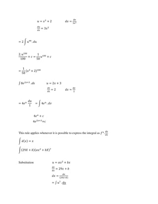
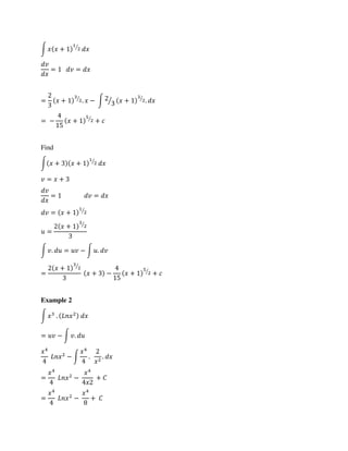
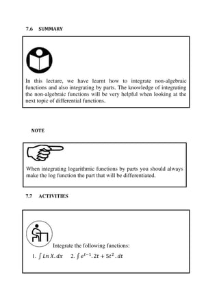
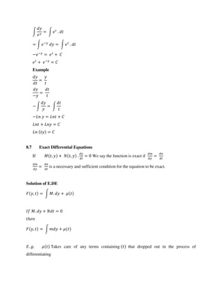
![7.3 Integration of non-algebraic functions.
Recall from the differentiation of non-algebraic functions:
If =
=
And
if = then
=
7.1.1 Exponential Rule
∫ . = +
∫ ′ �
= �
+
7.1.2 Logarithmic rule
∫ = +
∫
�′
�
= + >
| | + [ = ]
Example 1
∫
Using the exponential rule,
∫ = +
Example 2
∫ +](https://image.slidesharecdn.com/ees300module-181201121150/85/Ees-300-72-320.jpg)
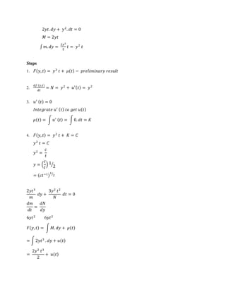
![∫
+
. = ∫
( )
. = +
= + +
Example 3
∫( − −
+ ⁄ )
= ∫ . − ∫ −
. + ∫ ⁄ .
= ∫ . = + . + −
+ +
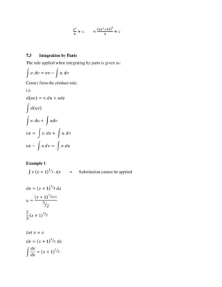
7.4 Integration by substitution
Used if appropriate
∫ . . = ∫ . = +
Comes from chain rule
= . = . =
∫ [ . ] = +
e.g.
∫ . + = = +
=](https://image.slidesharecdn.com/ees300module-181201121150/85/Ees-300-73-320.jpg)
![=
∫ = ∫ =
= +
=
+
+ = + + [ + ]
+ +
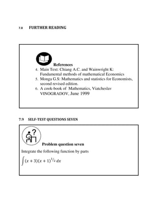
Definite integral after substitution
∫
+
.
= +
= =
∫
∫ = [ + ]
= .
= + = + =
=
= + =](https://image.slidesharecdn.com/ees300module-181201121150/85/Ees-300-74-320.jpg)
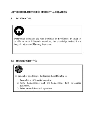
![[Lnv + ] = | | − Ln| |
*Ensure you change the limits.
Definite Integral as on area under the curve
=
=
=
0
∫ . = [ + ]
∫ . = − ∫ .
∫ =
∫ = ∫ .
∫ − = − ∫
∫ + = ∫ + .](https://image.slidesharecdn.com/ees300module-181201121150/85/Ees-300-75-320.jpg)
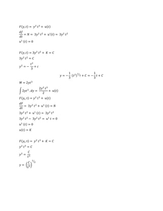
![To solve, assume = . Whats ?
The solution is the particular integral that ensures that A has a definite value,
When = � −
+ ⁄
= � + ⁄ � = − ⁄
= [ − ⁄ ] −
+ ⁄
8.6 Separable differential equations
These are equations that can be specifically separated into two parts, one a derivative of one
variable and the other a derivative of another variable. For example:
+ =
. + =
∫ . + ∫ =
Example
. = −�
∫ = ∫
= − +
= − +
= −
� =
Then
Y = Αe−at
− General solution
At t =
= Αe−
= Α
= −
−](https://image.slidesharecdn.com/ees300module-181201121150/85/Ees-300-85-320.jpg)
![= +
= ⁄
= ⁄
=
[ =] .
= +
= . . = → .
e.g.
= =
= → − . .
→ � ℎ .
8.8 Non linear D.E of 1st
order 1st
degree
appears in a higher power or lower power not equal to e.g.
+ =
Separable function e.g.
− =
+ . =
+ =
+ − =
−
+
−
−
=
∫
−
+ ∫ =
∫ = − ∫
+ = − +
= − +
= − +
⁄](https://image.slidesharecdn.com/ees300module-181201121150/85/Ees-300-91-320.jpg)
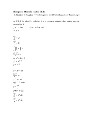
![= ,
= .
= . , = ,
= . , = ,
= . , = ,
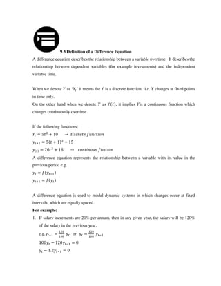
9.5 General solution for a Homogenous first order difference equation
+ − . =
If we get the income for years , , , , in terms of we will have:
+ = . =
= .
= . [ ] = . [ . ] .
= . [ ] = . [ . ]
= .
In general
= . −
Assume = = ,
= . −
= . ,
= . ,
= , .
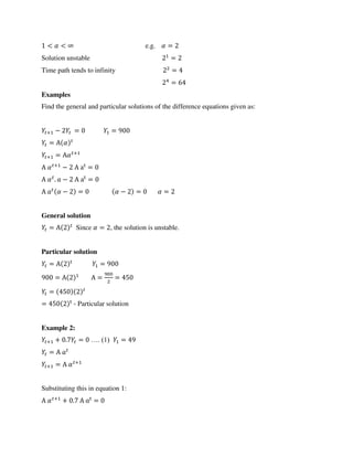
General and particular solutions of difference equations
We have shown that:
− . − = can be generalized as:
= . −
…………………………1](https://image.slidesharecdn.com/ees300module-181201121150/85/Ees-300-97-320.jpg)
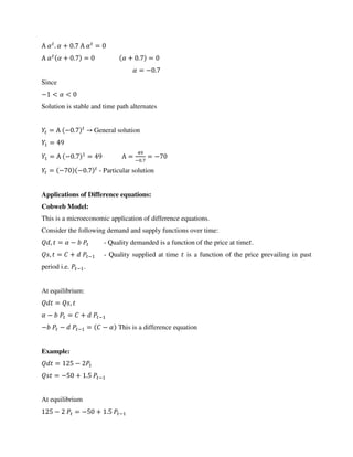
![This can be rewritten as:
= . . −
……………........2
= . −
. . . ………………………3
Since is a constant, . −
is also a constant, we can combine them into one constant to be
represented as � so that equation 3 becomes:
= � . = �. . ……………………4
. is also a constant. If we represent it with a small ′�′ we can have equation 4 written as:
= Α. � …………………………………5
This is called a general solution where ′�′ will be determined from the difference equation.
When we evaluate equation 5 at the given values of , and specific values of ′Α′we get a
particular solution.
Example:
Assume + = .
a) Find the general solution.
b) If = , find the particular solution.
c) Evaluate , , .
Solution
a) = Α �
+ = Α +
if + − . = then we can substitute this into equation of & + to
get:
Α � +
− . Α α t
=
Α � � − . Α � =
Α αt
α − . Ααt
=
Α at [α − . ] =](https://image.slidesharecdn.com/ees300module-181201121150/85/Ees-300-98-320.jpg)
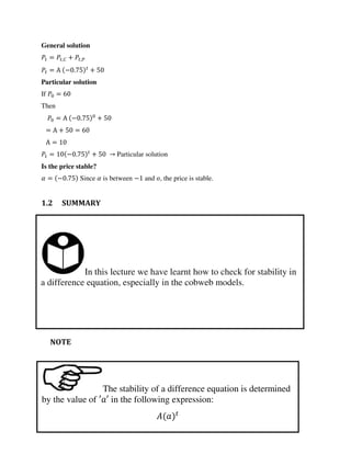
![+ = − +
→ . − + =
Since this is a non-homogenous difference equation, the solution will have two parts.
= . + Ι
= ,� + ,�
Find the Complementary functions:
+ . − =
= Α �
− = Α � −
Α � + . Α � −
=
Α � + . Α � . �−
=
Α � [ − . �− ] =
+
.
�
=
= −
.
�
� = −
.
= − .
Therefore:
,� = Α − .
Particular Integral
Since the right hand side is a constant, the
,� =
− ,� =
Hence: in + . − =
+ . =
. =
= =
, =](https://image.slidesharecdn.com/ees300module-181201121150/85/Ees-300-108-320.jpg)
![• 5x1 + 2x2 ≤ 50 ( Total time of machine M2)
• 2x1 + 6x2 ≤ 60 ( Total time of machine M3)
• X1, x2≥ 0 [ Non-Negativity constraint)
• X1= X2 =
Solution to self test three
• Y=4
• X=2
• Z==44
Solution to self test four
X=6 Y=4 Z=2
Solution to self test five
• = [
−
−
−
]
• |H | <
• |H | >
• |H | <
• Z=Concave
Solution to self test six
• X1 =2; X2 = 10:
•
Solution to self test seven
• = +
• = =
• = + ⁄](https://image.slidesharecdn.com/ees300module-181201121150/85/Ees-300-113-320.jpg)
![• =
+ ⁄
• ∫ . = − ∫ .
• =
+ ⁄
+ − + ⁄
+
Solution to self test eight
1. ∫ . = ∫ .
+ = +
− =
− =
= +
= √ +
±
= � −
+
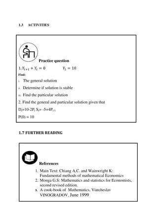
Solution to self test nine
Complementary function
,� = Α (− ⁄ )
Particular Integral
Since the right hand side = . , the general form of
, = .
+ ,� = . +
= . .
Substituting this in the original difference equation it will be:
+ + = .
. . +
+ . = .
. . . + . = .
. . [ . + ] = .
Divide all through by . , we get](https://image.slidesharecdn.com/ees300module-181201121150/85/Ees-300-114-320.jpg)
![[ . + ] =
. =
=
.
=
Therefore:
,� = . .
General solution:
= ,� + ,�
= Α (− ⁄ ) + .
Particular solution
=
= Α (− ⁄ ) + . =
Α + = Α =
Yt = (− ⁄ )
t
+ .
Solution to self-test ten
Pt = A − t
+
Solution is stable](https://image.slidesharecdn.com/ees300module-181201121150/85/Ees-300-115-320.jpg)