Download to read offline
![Lecture Notes CMSC 251
Lecture 2: Analyzing Algorithms: The 2-d Maxima Problem
(Thursday, Jan 29, 1998)
Read: Chapter 1 in CLR.
Analyzing Algorithms: In order to design good algorithms, we must first agree the criteria for measuring
algorithms. The emphasis in this course will be on the design of efficient algorithm, and hence we
will measure algorithms in terms of the amount of computational resources that the algorithm requires.
These resources include mostly running time and memory. Depending on the application, there may
be other elements that are taken into account, such as the number disk accesses in a database program
or the communication bandwidth in a networking application.
In practice there are many issues that need to be considered in the design algorithms. These include
issues such as the ease of debugging and maintaining the final software through its life-cycle. Also,
one of the luxuries we will have in this course is to be able to assume that we are given a clean, fully-
specified mathematical description of the computational problem. In practice, this is often not the case,
and the algorithm must be designed subject to only partial knowledge of the final specifications. Thus,
in practice it is often necessary to design algorithms that are simple, and easily modified if problem
parameters and specifications are slightly modified. Fortunately, most of the algorithms that we will
discuss in this class are quite simple, and are easy to modify subject to small problem variations.
Model of Computation: Another goal that we will have in this course is that our analyses be as independent
as possible of the variations in machine, operating system, compiler, or programming language. Unlike
programs, algorithms to be understood primarily by people (i.e. programmers) and not machines. Thus
gives us quite a bit of flexibility in how we present our algorithms, and many low-level details may be
omitted (since it will be the job of the programmer who implements the algorithm to fill them in).
But, in order to say anything meaningful about our algorithms, it will be important for us to settle
on a mathematical model of computation. Ideally this model should be a reasonable abstraction of a
standard generic single-processor machine. We call this model a random access machine or RAM.
A RAM is an idealized machine with an infinitely large random-access memory. Instructions are exe-
cuted one-by-one (there is no parallelism). Each instruction involves performing some basic operation
on two values in the machines memory (which might be characters or integers; let’s avoid floating
point for now). Basic operations include things like assigning a value to a variable, computing any
basic arithmetic operation (+, −, ∗, integer division) on integer values of any size, performing any
comparison (e.g. x ≤ 5) or boolean operations, accessing an element of an array (e.g. A[10]). We
assume that each basic operation takes the same constant time to execute.
This model seems to go a good job of describing the computational power of most modern (nonparallel)
machines. It does not model some elements, such as efficiency due to locality of reference, as described
in the previous lecture. There are some “loop-holes” (or hidden ways of subverting the rules) to beware
of. For example, the model would allow you to add two numbers that contain a billion digits in constant
time. Thus, it is theoretically possible to derive nonsensical results in the form of efficient RAM
programs that cannot be implemented efficiently on any machine. Nonetheless, the RAM model seems
to be fairly sound, and has done a good job of modeling typical machine technology since the early
60’s.
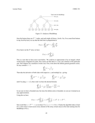
Example: 2-dimension Maxima: Rather than jumping in with all the definitions, let us begin the discussion
of how to analyze algorithms with a simple problem, called 2-dimension maxima. To motivate the
problem, suppose that you want to buy a car. Since you’re a real swinger you want the fastest car
around, so among all cars you pick the fastest. But cars are expensive, and since you’re a swinger on
a budget, you want the cheapest. You cannot decide which is more important, speed or price, but you
know that you definitely do NOT want to consider a car if there is another car that is both faster and
3](https://image.slidesharecdn.com/251-alogarithmslects-230702222135-b89653fc/85/251-Alogarithms-Lects-pdf-3-320.jpg)
![Lecture Notes CMSC 251
cheaper. We say that the fast, cheap car dominates the slow, expensive car relative to your selection
criteria. So, given a collection of cars, we want to list those that are not dominated by any other.
Here is how we might model this as a formal problem. Let a point p in 2-dimensional space be given
by its integer coordinates, p = (p.x, p.y). A point p is said to dominated by point q if p.x ≤ q.x and
p.y ≤ q.y. Given a set of n points, P = {p1, p2, . . . , pn} in 2-space a point is said to be maximal if it
is not dominated by any other point in P.
The car selection problem can be modeled in this way. If for each car we associated (x, y) values where
x is the speed of the car, and y is the negation of the price (thus high y values mean cheap cars), then
the maximal points correspond to the fastest and cheapest cars.
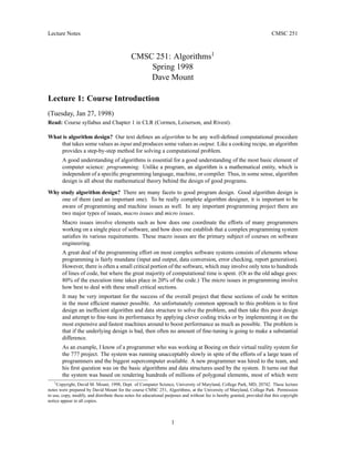
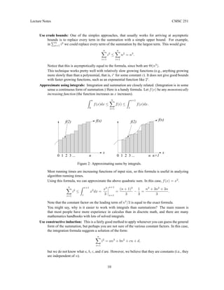
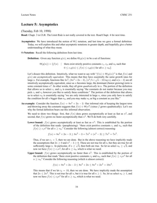
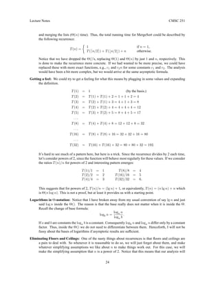
2-dimensional Maxima: Given a set of points P = {p1, p2, . . . , pn} in 2-space, each represented by
its x and y integer coordinates, output the set of the maximal points of P, that is, those points pi,
such that pi is not dominated by any other point of P. (See the figure below.)
(2,5)
2 4 6 8 10
2
4
6
8
10
12 14
(9,10)
(13,3)
(15,7)
(14,10)
(12,12)
(7,13)
(11,5)
(4,11)
(7,7)
(5,1)
(4,4)
14
12
16
Figure 1: Maximal Points.
Observe that our description of the problem so far has been at a fairly mathematical level. For example,
we have intentionally not discussed issues as to how points are represented (e.g., using a structure with
records for the x and y coordinates, or a 2-dimensional array) nor have we discussed input and output
formats. These would normally be important in a software specification. However, we would like to
keep as many of the messy issues out since they would just clutter up the algorithm.
Brute Force Algorithm: To get the ball rolling, let’s just consider a simple brute-force algorithm, with no
thought to efficiency. Here is the simplest one that I can imagine. Let P = {p1, p2, . . . , pn} be the
initial set of points. For each point pi, test it against all other points pj. If pi is not dominated by any
other point, then output it.
This English description is clear enough that any (competent) programmer should be able to implement
it. However, if you want to be a bit more formal, it could be written in pseudocode as follows:
Brute Force Maxima
Maxima(int n, Point P[1..n]) { // output maxima of P[0..n-1]
for i = 1 to n {
maximal = true; // P[i] is maximal by default
for j = 1 to n {
if (i != j) and (P[i].x <= P[j].x) and (P[i].y <= P[j].y) {
4](https://image.slidesharecdn.com/251-alogarithmslects-230702222135-b89653fc/85/251-Alogarithms-Lects-pdf-4-320.jpg)
![Lecture Notes CMSC 251
maximal = false; // P[i] is dominated by P[j]
break;
}
}
if (maximal) output P[i]; // no one dominated...output
}
}
There are no formal rules to the syntax of this pseudocode. In particular, do not assume that more
detail is better. For example, I omitted type specifications for the procedure Maxima and the variable
maximal, and I never defined what a Point data type is, since I felt that these are pretty clear
from context or just unimportant details. Of course, the appropriate level of detail is a judgement call.
Remember, algorithms are to be read by people, and so the level of detail depends on your intended
audience. When writing pseudocode, you should omit details that detract from the main ideas of the
algorithm, and just go with the essentials.
You might also notice that I did not insert any checking for consistency. For example, I assumed that
the points in P are all distinct. If there is a duplicate point then the algorithm may fail to output even
a single point. (Can you see why?) Again, these are important considerations for implementation, but
we will often omit error checking because we want to see the algorithm in its simplest form.
Correctness: Whenever you present an algorithm, you should also present a short argument for its correct-
ness. If the algorithm is tricky, then this proof should contain the explanations of why the tricks works.
In a simple case like the one above, there almost nothing that needs to be said. We simply implemented
the definition: a point is maximal if no other point dominates it.
Running Time Analysis: The main purpose of our mathematical analyses will be be measure the execution
time (and sometimes the space) of an algorithm. Obviously the running time of an implementation of
the algorithm would depend on the speed of the machine, optimizations of the compiler, etc. Since we
want to avoid these technology issues and treat algorithms as mathematical objects, we will only focus
on the pseudocode itself. This implies that we cannot really make distinctions between algorithms
whose running times differ by a small constant factor, since these algorithms may be faster or slower
depending on how well they exploit the particular machine and compiler. How small is small? To
make matters mathematically clean, let us just ignore all constant factors in analyzing running times.
We’ll see later why even with this big assumption, we can still make meaningful comparisons between
algorithms.
In this case we might measure running time by counting the number of steps of pseudocode that are
executed, or the number of times that an element of P is accessed, or the number of comparisons that
are performed.
Running time depends on input size. So we will define running time in terms of a function of input
size. Formally, the input size is defined to be the number of characters in the input file, assuming some
reasonable encoding of inputs (e.g. numbers are represented in base 10 and separated by a space).
However, we will usually make the simplifying assumption that each number is of some constant
maximum length (after all, it must fit into one computer word), and so the input size can be estimated
up to constant factor by the parameter n, that is, the length of the array P.
Also, different inputs of the same size may generally result in different execution times. (For example,
in this problem, the number of times we execute the inner loop before breaking out depends not only on
the size of the input, but the structure of the input.) There are two common criteria used in measuring
running times:
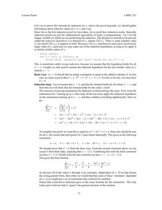
Worst-case time: is the maximum running time over all (legal) inputs of size n? Let I denote a legal
input instance, and let |I| denote its length, and let T(I) denote the running time of the algorithm
5](https://image.slidesharecdn.com/251-alogarithmslects-230702222135-b89653fc/85/251-Alogarithms-Lects-pdf-5-320.jpg)
![Lecture Notes CMSC 251
on input I.
Tworst(n) = max
|I|=n
T(I).
Average-case time: is the average running time over all inputs of size n? More generally, for each
input I, let p(I) denote the probability of seeing this input. The average-case running time is the
weight sum of running times, with the probability being the weight.
Tavg(n) =
X
|I|=n
p(I)T(I).
We will almost always work with worst-case running time. This is because for many of the problems
we will work with, average-case running time is just too difficult to compute, and it is difficult to specify
a natural probability distribution on inputs that are really meaningful for all applications. It turns out
that for most of the algorithms we will consider, there will be only a constant factor difference between
worst-case and average-case times.
Running Time of the Brute Force Algorithm: Let us agree that the input size is n, and for the running
time we will count the number of time that any element of P is accessed. Clearly we go through the
outer loop n times, and for each time through this loop, we go through the inner loop n times as well.
The condition in the if-statement makes four accesses to P. (Under C semantics, not all four need be
evaluated, but let’s ignore this since it will just complicate matters). The output statement makes two
accesses (to P[i].x and P[i].y) for each point that is output. In the worst case every point is maximal
(can you see how to generate such an example?) so these two access are made for each time through
the outer loop.
Thus we might express the worst-case running time as a pair of nested summations, one for the i-loop
and the other for the j-loop:
T(n) =
n
X
i=1
2 +
n
X
j=1
4
.
These are not very hard summations to solve.
Pn
j=1 4 is just 4n, and so
T(n) =
n
X
i=1
(4n + 2) = (4n + 2)n = 4n2
+ 2n.
As mentioned before we will not care about the small constant factors. Also, we are most interested in
what happens as n gets large. Why? Because when n is small, almost any algorithm is fast enough.
It is only for large values of n that running time becomes an important issue. When n is large, the n2
term will be much larger than the n term, and so it will dominate the running time. We will sum this
analysis up by simply saying that the worst-case running time of the brute force algorithm is Θ(n2
).
This is called the asymptotic growth rate of the function. Later we will discuss more formally what
this notation means.
Summations: (This is covered in Chapter 3 of CLR.) We saw that this analysis involved computing a sum-
mation. Summations should be familiar from CMSC 150, but let’s review a bit here. Given a finite
sequence of values a1, a2, . . . , an, their sum a1 +a2 +· · ·+an can be expressed in summation notation
as
n
X
i=1
ai.
If n = 0, then the value of the sum is the additive identity, 0. There are a number of simple algebraic
facts about sums. These are easy to verify by simply writing out the summation and applying simple
6](https://image.slidesharecdn.com/251-alogarithmslects-230702222135-b89653fc/85/251-Alogarithms-Lects-pdf-6-320.jpg)
![Lecture Notes CMSC 251
high school algebra. If c is a constant (does not depend on the summation index i) then
n
X
i=1
cai = c
n
X
i=1
ai and
n
X
i=1
(ai + bi) =
n
X
i=1
ai +
n
X
i=1
bi.
There are some particularly important summations, which you should probably commit to memory (or
at least remember their asymptotic growth rates). If you want some practice with induction, the first
two are easy to prove by induction.
Arithmetic Series: For n ≥ 0,
n
X
i=1
i = 1 + 2 + · · · + n =
n(n + 1)
2
= Θ(n2
).
Geometric Series: Let x 6= 1 be any constant (independent of i), then for n ≥ 0,
n
X
i=0
xi
= 1 + x + x2
+ · · · + xn
=
xn+1
− 1
x − 1
.
If 0 < x < 1 then this is Θ(1), and if x > 1, then this is Θ(xn
).
Harmonic Series: This arises often in probabilistic analyses of algorithms. For n ≥ 0,
Hn =
n
X
i=1
1
i
= 1 +
1
2
+
1
3
+ · · · +
1
n
≈ ln n = Θ(ln n).
Lecture 3: Summations and Analyzing Programs with Loops
(Tuesday, Feb 3, 1998)
Read: Chapt. 3 in CLR.
Recap: Last time we presented an algorithm for the 2-dimensional maxima problem. Recall that the algo-
rithm consisted of two nested loops. It looked something like this:
Brute Force Maxima
Maxima(int n, Point P[1..n]) {
for i = 1 to n {
...
for j = 1 to n {
...
...
}
}
We were interested in measuring the worst-case running time of this algorithm as a function of the
input size, n. The stuff in the “...” has been omitted because it is unimportant for the analysis.
Last time we counted the number of times that the algorithm accessed a coordinate of any point. (This
was only one of many things that we could have chosen to count.) We showed that as a function of n
in the worst case this quantity was
T(n) = 4n2
+ 2n.
7](https://image.slidesharecdn.com/251-alogarithmslects-230702222135-b89653fc/85/251-Alogarithms-Lects-pdf-7-320.jpg)
![Lecture Notes CMSC 251
(b)
sweep line
sweep line
(a)
4
2
(2,5)
(13,3)
(9,10)
(4,11)
(3,13)
(10,5)
(7,7) (15,7)
(14,10)
(12,12)
(5,1)
(4,4)
14
12
16
14
12
10
8
6
4
2
10
8
6 6
(2,5)
(13,3)
(9,10)
(4,11)
(3,13)
(10,5)
(7,7) (15,7)
(14,10)
(12,12)
8 10
2
4
6
8
10
12 14 16
12
14
(4,4)
(5,1)
4
2
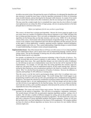
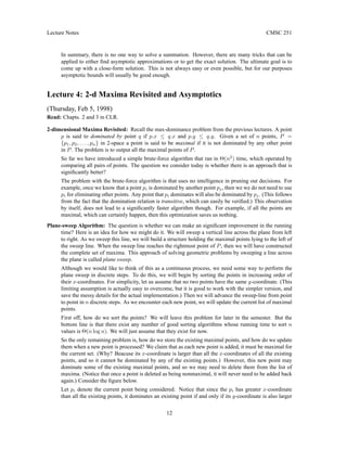
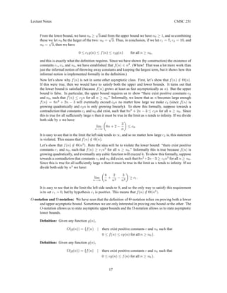
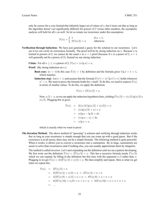
Figure 3: Plane sweep algorithm for 2-d maxima.
(or equal). Thus, among the existing maximal points, we want to find those having smaller (or equal)
y-coordinate, and eliminate them.
At this point, we need to make an important observation about how maximal points are ordered with
respect to the x- and y-coordinates. As we read maximal points from left to right (in order of increasing
x-coordinates) the y-coordinates appear in decreasing order. Why is this so? Suppose to the contrary,
that we had two maximal points p and q, with p.x ≥ q.x but p.y ≥ q.y. Then it would follow that q is
dominated by p, and hence it is not maximal, a contradiction.
This is nice, because it implies that if we store the existing maximal points in a list, the points that
pi dominates (if any) will all appear at the end of this list. So we have to scan this list to find the
breakpoint between the maximal and dominated points. The question is how do we do this?
I claim that we can simply scan the list linearly. But we must do the scan in the proper direction for
the algorithm to be efficient. Which direction should we scan the list of current maxima? From left
to right, until finding the first point that is not dominated, or from right to left, until finding the first
point that is dominated? Stop here and think about it for a moment. If you can answer this question
correctly, then it says something about your intuition for designing efficient algorithms. Let us assume
that we are trying to optimize worst-case performance.
The correct answer is to scan the list from left to right. Here is why. If you only encounter one point
in the scan, then the scan will always be very efficient. The danger is that you may scan many points
before finding the proper breakpoint. If we scan the list from left to right, then every point that we
encounter whose y-coordinate is less than pi’s will be dominated, and hence it will be eliminated from
the computation forever. We will never have to scan this point again. On the other hand, if we scan
from left to right, then in the worst case (consider when all the points are maximal) we may rescan the
same points over and over again. This will lead to an Θ(n2
) algorithm
Now we can give the pseudocode for the final plane sweep algorithm. Since we add maximal points
onto the end of the list, and delete them from the end of the list, we can use a stack to store the maximal
points, where the top of the stack contains the point with the highest x-coordinate. Let S denote this
stack. The top element of the stack is denoted S.top. Popping the stack means removing the top
element.
Plane Sweep Maxima
Maxima2(int n, Point P[1..n]) {
13](https://image.slidesharecdn.com/251-alogarithmslects-230702222135-b89653fc/85/251-Alogarithms-Lects-pdf-13-320.jpg)
![Lecture Notes CMSC 251
Sort P in ascending order by x-coordinate;
S = empty; // initialize stack of maxima
for i = 1 to n do { // add points in order of x-coordinate
while (S is not empty and S.top.y <= P[i].y)
Pop(S); // remove points that P[i] dominates
Push(S, P[i]); // add P[i] to stack of maxima
}
output the contents of S;
}
Why is this algorithm correct? The correctness follows from the discussion up to now. The most
important element was that since the current maxima appear on the stack in decreasing order of x-
coordinates (as we look down from the top of the stack), they occur in increasing order of y-coordinates.
Thus, as soon as we find the last undominated element in the stack, it follows that everyone else on the
stack is undominated.
Analysis: This is an interesting program to analyze, primarily because the techniques that we discussed in
the last lecture do not apply readily here. I claim that after the sorting (which we mentioned takes
Θ(n log n) time), the rest of the algorithm only takes Θ(n) time. In particular, we have two nested
loops. The outer loop is clearly executed n times. The inner while-loop could be iterated up to n − 1
times in the worst case (in particular, when the last point added dominates all the others). So, it seems
that though we have n(n − 1) for a total of Θ(n2
).
However, this is a good example of how not to be fooled by analyses that are too simple minded.
Although it is true that the inner while-loop could be executed as many as n − 1 times any one time
through the outer loop, over the entire course of the algorithm we claim that it cannot be executed
more than n times. Why is this? First observe that the total number of elements that have ever been
pushed onto the stack is at most n, since we execute exactly one Push for each time through the outer
for-loop. Also observe that every time we go through the inner while-loop, we must pop an element off
the stack. It is impossible to pop more elements off the stack than are ever pushed on. Therefore, the
inner while-loop cannot be executed more than n times over the entire course of the algorithm. (Make
sure that you believe the argument before going on.)
Therefore, since the total number of iterations of the inner while-loop is n, and since the total number
of iterations in the outer for-loop is n, the total running time of the algorithm is Θ(n).
Is this really better? How much of an improvement is this plane-sweep algorithm over the brute-force al-
gorithm? Probably the most accurate way to find out would be to code the two up, and compare their
running times. But just to get a feeling, let’s look at the ratio of the running times. (We have ignored
constant factors, but we’ll see that they cannot play a very big role.)
We have argued that the brute-force algorithm runs in Θ(n2
) time, and the improved plane-sweep
algorithm runs in Θ(n log n) time. What is the base of the logarithm? It turns out that it will not matter
for the asymptotics (we’ll show this later), so for concreteness, let’s assume logarithm base 2, which
we’ll denote as lg n. The ratio of the running times is:
n2
n lg n
=
n
lg n
.
For relatively small values of n (e.g. less than 100), both algorithms are probably running fast enough
that the difference will be practically negligible. On larger inputs, say, n = 1, 000, the ratio of n to
lg n is about 1000/10 = 100, so there is a 100-to-1 ratio in running times. Of course, we have not
considered the constant factors. But since neither algorithm makes use of very complex constructs, it
is hard to imagine that the constant factors will differ by more than, say, a factor of 10. For even larger
14](https://image.slidesharecdn.com/251-alogarithmslects-230702222135-b89653fc/85/251-Alogarithms-Lects-pdf-14-320.jpg)
![Lecture Notes CMSC 251
Lecture 6: Divide and Conquer and MergeSort
(Thursday, Feb 12, 1998)
Read: Chapt. 1 (on MergeSort) and Chapt. 4 (on recurrences).
Divide and Conquer: The ancient Roman politicians understood an important principle of good algorithm
design (although they were probably not thinking about algorithms at the time). You divide your
enemies (by getting them to distrust each other) and then conquer them piece by piece. This is called
divide-and-conquer. In algorithm design, the idea is to take a problem on a large input, break the input
into smaller pieces, solve the problem on each of the small pieces, and then combine the piecewise
solutions into a global solution. But once you have broken the problem into pieces, how do you solve
these pieces? The answer is to apply divide-and-conquer to them, thus further breaking them down.
The process ends when you are left with such tiny pieces remaining (e.g. one or two items) that it is
trivial to solve them.
Summarizing, the main elements to a divide-and-conquer solution are
• Divide (the problem into a small number of pieces),
• Conquer (solve each piece, by applying divide-and-conquer recursively to it), and
• Combine (the pieces together into a global solution).
There are a huge number computational problems that can be solved efficiently using divide-and-
conquer. In fact the technique is so powerful, that when someone first suggests a problem to me,
the first question I usually ask (after what is the brute-force solution) is “does there exist a divide-and-
conquer solution for this problem?”
Divide-and-conquer algorithms are typically recursive, since the conquer part involves invoking the
same technique on a smaller subproblem. Analyzing the running times of recursive programs is rather
tricky, but we will show that there is an elegant mathematical concept, called a recurrence, which is
useful for analyzing the sort of recursive programs that naturally arise in divide-and-conquer solutions.
For the next couple of lectures we will discuss some examples of divide-and-conquer algorithms, and
how to analyze them using recurrences.
MergeSort: The first example of a divide-and-conquer algorithm which we will consider is perhaps the best
known. This is a simple and very efficient algorithm for sorting a list of numbers, called MergeSort.
We are given an sequence of n numbers A, which we will assume is stored in an array A[1 . . . n]. The
objective is to output a permutation of this sequence, sorted in increasing order. This is normally done
by permuting the elements within the array A.
How can we apply divide-and-conquer to sorting? Here are the major elements of the MergeSort
algorithm.
Divide: Split A down the middle into two subsequences, each of size roughly n/2.
Conquer: Sort each subsequence (by calling MergeSort recursively on each).
Combine: Merge the two sorted subsequences into a single sorted list.
The dividing process ends when we have split the subsequences down to a single item. An sequence
of length one is trivially sorted. The key operation where all the work is done is in the combine stage,
which merges together two sorted lists into a single sorted list. It turns out that the merging process is
quite easy to implement.
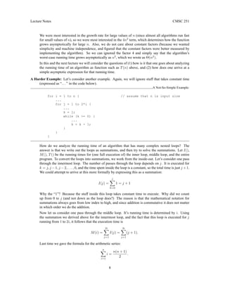
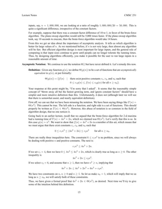
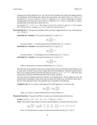
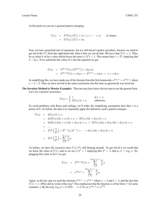
The following figure gives a high-level view of the algorithm. The “divide” phase is shown on the left.
It works top-down splitting up the list into smaller sublists. The “conquer and combine” phases are
shown on the right. They work bottom-up, merging sorted lists together into larger sorted lists.
20](https://image.slidesharecdn.com/251-alogarithmslects-230702222135-b89653fc/85/251-Alogarithms-Lects-pdf-20-320.jpg)
![Lecture Notes CMSC 251
7 5 2 4 1 6 3 0 output:
input:
split merge
2 4 5 7
5 7
0 1 3 6
0 3
0 1 2 3 4 5 6 7
7
1 6
2 4
0
3
6
1
4
2
5
7
5
7 5 2 4 1 6 3 0
3 0
1 6
2 4
7 5
0
3
6
1
4
2
Figure 4: MergeSort.
MergeSort: Let’s design the algorithm top-down. We’ll assume that the procedure that merges two sorted
list is available to us. We’ll implement it later. Because the algorithm is called recursively on sublists,
in addition to passing in the array itself, we will pass in two indices, which indicate the first and last
indices of the subarray that we are to sort. The call MergeSort(A, p, r) will sort the subarray
A[p..r] and return the sorted result in the same subarray.
Here is the overview. If r = p, then this means that there is only one element to sort, and we may return
immediately. Otherwise (if p r) there are at least two elements, and we will invoke the divide-and-
conquer. We find the index q, midway between p and r, namely q = (p + r)/2 (rounded down to the
nearest integer). Then we split the array into subarrays A[p..q] and A[q + 1..r]. (We need to be careful
here. Why would it be wrong to do A[p..q − 1] and A[q..r]? Suppose r = p + 1.) Call MergeSort
recursively to sort each subarray. Finally, we invoke a procedure (which we have yet to write) which
merges these two subarrays into a single sorted array.
MergeSort
MergeSort(array A, int p, int r) {
if (p r) { // we have at least 2 items
q = (p + r)/2
MergeSort(A, p, q) // sort A[p..q]
MergeSort(A, q+1, r) // sort A[q+1..r]
Merge(A, p, q, r) // merge everything together
}
}
Merging: All that is left is to describe the procedure that merges two sorted lists. Merge(A, p, q, r)
assumes that the left subarray, A[p..q], and the right subarray, A[q + 1..r], have already been sorted.
We merge these two subarrays by copying the elements to a temporary working array called B. For
convenience, we will assume that the array B has the same index range A, that is, B[p..r]. (One nice
thing about pseudocode, is that we can make these assumptions, and leave them up to the programmer
to figure out how to implement it.) We have to indices i and j, that point to the current elements of
each subarray. We move the smaller element into the next position of B (indicated by index k) and
then increment the corresponding index (either i or j). When we run out of elements in one array, then
we just copy the rest of the other array into B. Finally, we copy the entire contents of B back into A.
(The use of the temporary array is a bit unpleasant, but this is impossible to overcome entirely. It is one
of the shortcomings of MergeSort, compared to some of the other efficient sorting algorithms.)
In case you are not aware of C notation, the operator i++ returns the current value of i, and then
increments this variable by one.
Merge
Merge(array A, int p, int q, int r) { // merges A[p..q] with A[q+1..r]
21](https://image.slidesharecdn.com/251-alogarithmslects-230702222135-b89653fc/85/251-Alogarithms-Lects-pdf-21-320.jpg)
![Lecture Notes CMSC 251
array B[p..r]
i = k = p // initialize pointers
j = q+1
while (i = q and j = r) { // while both subarrays are nonempty
if (A[i] = A[j]) B[k++] = A[i++] // copy from left subarray
else B[k++] = A[j++] // copy from right subarray
}
while (i = q) B[k++] = A[i++] // copy any leftover to B
while (j = r) B[k++] = A[j++]
for i = p to r do A[i] = B[i] // copy B back to A
}
This completes the description of the algorithm. Observe that of the last two while-loops in the Merge
procedure, only one will be executed. (Do you see why?)
If you find the recursion to be a bit confusing. Go back and look at the earlier figure. Convince yourself
that as you unravel the recursion you are essentially walking through the tree (the recursion tree) shown
in the figure. As calls are made you walk down towards the leaves, and as you return you are walking
up towards the root. (We have drawn two trees in the figure, but this is just to make the distinction
between the inputs and outputs clearer.)
Discussion: One of the little tricks in improving the running time of this algorithm is to avoid the constant
copying from A to B and back to A. This is often handled in the implementation by using two arrays,
both of equal size. At odd levels of the recursion we merge from subarrays of A to a subarray of B. At
even levels we merge from from B to A. If the recursion has an odd number of levels, we may have to
do one final copy from B back to A, but this is faster than having to do it at every level. Of course, this
only improves the constant factors; it does not change the asymptotic running time.
Another implementation trick to speed things by a constant factor is that rather than driving the divide-
and-conquer all the way down to subsequences of size 1, instead stop the dividing process when the
sequence sizes fall below constant, e.g. 20. Then invoke a simple Θ(n2
) algorithm, like insertion sort
on these small lists. Often brute force algorithms run faster on small subsequences, because they do
not have the added overhead of recursion. Note that since they are running on subsequences of size at
most 20, the running times is Θ(202
) = Θ(1). Thus, this will not affect the overall asymptotic running
time.
It might seem at first glance that it should be possible to merge the lists “in-place”, without the need
for additional temporary storage. The answer is that it is, but it no one knows how to do it without
destroying the algorithm’s efficiency. It turns out that there are faster ways to sort numbers in-place,
e.g. using either HeapSort or QuickSort.
Here is a subtle but interesting point to make regarding this sorting algorithm. Suppose that in the if-
statement above, we have A[i] = A[j]. Observe that in this case we copy from the left sublist. Would
it have mattered if instead we had copied from the right sublist? The simple answer is no—since the
elements are equal, they can appear in either order in the final sublist. However there is a subtler reason
to prefer this particular choice. Many times we are sorting data that does not have a single attribute,
but has many attributes (name, SSN, grade, etc.) Often the list may already have been sorted on one
attribute (say, name). If we sort on a second attribute (say, grade), then it would be nice if people with
same grade are still sorted by name. A sorting algorithm that has the property that equal items will
appear in the final sorted list in the same relative order that they appeared in the initial input is called a
stable sorting algorithm. This is a nice property for a sorting algorithm to have. By favoring elements
from the left sublist over the right, we will be preserving the relative order of elements. It can be shown
that as a result, MergeSort is a stable sorting algorithm. (This is not immediate, but it can be proved by
induction.)
22](https://image.slidesharecdn.com/251-alogarithmslects-230702222135-b89653fc/85/251-Alogarithms-Lects-pdf-22-320.jpg)
![Lecture Notes CMSC 251
Analysis: What remains is to analyze the running time of MergeSort. First let us consider the running time
of the procedure Merge(A, p, q, r). Let n = r − p + 1 denote the total length of both the left
and right subarrays. What is the running time of Merge as a function of n? The algorithm contains four
loops (none nested in the other). It is easy to see that each loop can be executed at most n times. (If
you are a bit more careful you can actually see that all the while-loops together can only be executed n
times in total, because each execution copies one new element to the array B, and B only has space for
n elements.) Thus the running time to Merge n items is Θ(n). Let us write this without the asymptotic
notation, simply as n. (We’ll see later why we do this.)
Now, how do we describe the running time of the entire MergeSort algorithm? We will do this through
the use of a recurrence, that is, a function that is defined recursively in terms of itself. To avoid
circularity, the recurrence for a given value of n is defined in terms of values that are strictly smaller
than n. Finally, a recurrence has some basis values (e.g. for n = 1), which are defined explicitly.
Let’s see how to apply this to MergeSort. Let T(n) denote the worst case running time of MergeSort on
an array of length n. For concreteness we could count whatever we like: number of lines of pseudocode,
number of comparisons, number of array accesses, since these will only differ by a constant factor.
Since all of the real work is done in the Merge procedure, we will count the total time spent in the
Merge procedure.
First observe that if we call MergeSort with a list containing a single element, then the running time is a
constant. Since we are ignoring constant factors, we can just write T(n) = 1. When we call MergeSort
with a list of length n 1, e.g. Merge(A, p, r), where r−p+1 = n, the algorithm first computes
q = b(p + r)/2c. The subarray A[p..q], which contains q − p + 1 elements. You can verify (by some
tedious floor-ceiling arithmetic, or simpler by just trying an odd example and an even example) that is
of size dn/2e. Thus the remaining subarray A[q +1..r] has bn/2c elements in it. How long does it take
to sort the left subarray? We do not know this, but because dn/2e n for n 1, we can express this
as T(dn/2e). Similarly, we can express the time that it takes to sort the right subarray as T(bn/2c).
Finally, to merge both sorted lists takes n time, by the comments made above. In conclusion we have
T(n) =
1 if n = 1,
T(dn/2e) + T(bn/2c) + n otherwise.
Lecture 7: Recurrences
(Tuesday, Feb 17, 1998)
Read: Chapt. 4 on recurrences. Skip Section 4.4.
Divide and Conquer and Recurrences: Last time we introduced divide-and-conquer as a basic technique
for designing efficient algorithms. Recall that the basic steps in divide-and-conquer solution are (1)
divide the problem into a small number of subproblems, (2) solve each subproblem recursively, and (3)
combine the solutions to the subproblems to a global solution. We also described MergeSort, a sorting
algorithm based on divide-and-conquer.
Because divide-and-conquer is an important design technique, and because it naturally gives rise to
recursive algorithms, it is important to develop mathematical techniques for solving recurrences, either
exactly or asymptotically. To do this, we introduced the notion of a recurrence, that is, a recursively
defined function. Today we discuss a number of techniques for solving recurrences.
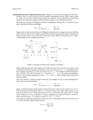
MergeSort Recurrence: Here is the recurrence we derived last time for MergeSort. Recall that T(n) is the
time to run MergeSort on a list of size n. We argued that if the list is of length 1, then the total sorting
time is a constant Θ(1). If n 1, then we must recursively sort two sublists, one of size dn/2e and
the other of size bn/2c, and the nonrecursive part took Θ(n) time for splitting the list (constant time)
23](https://image.slidesharecdn.com/251-alogarithmslects-230702222135-b89653fc/85/251-Alogarithms-Lects-pdf-23-320.jpg)
![Lecture Notes CMSC 251
Finally, in the recurrence T(n) = 4T(n/3) + n (which corresponds to Case 1), most of the work is
done at the leaf level of the recursion tree. This can be seen if you perform iteration on this recurrence,
the resulting summation is
n
log3 n
X
i=0
4
3
i
.
(You might try this to see if you get the same result.) Since 4/3 1, as we go deeper into the levels
of the tree, that is deeper into the summation, the terms are growing successively larger. The largest
contribution will be from the leaf level.
Lecture 9: Medians and Selection
(Tuesday, Feb 24, 1998)
Read: Todays material is covered in Sections 10.2 and 10.3. You are not responsible for the randomized
analysis of Section 10.2. Our presentation of the partitioning algorithm and analysis are somewhat different
from the ones in the book.
Selection: In the last couple of lectures we have discussed recurrences and the divide-and-conquer method
of solving problems. Today we will give a rather surprising (and very tricky) algorithm which shows
the power of these techniques.
The problem that we will consider is very easy to state, but surprisingly difficult to solve optimally.
Suppose that you are given a set of n numbers. Define the rank of an element to be one plus the
number of elements that are smaller than this element. Since duplicate elements make our life more
complex (by creating multiple elements of the same rank), we will make the simplifying assumption
that all the elements are distinct for now. It will be easy to get around this assumption later. Thus, the
rank of an element is its final position if the set is sorted. The minimum is of rank 1 and the maximum
is of rank n.
Of particular interest in statistics is the median. If n is odd then the median is defined to be the element
of rank (n + 1)/2. When n is even there are two natural choices, namely the elements of ranks n/2
and (n/2) + 1. In statistics it is common to return the average of these two elements. We will define
the median to be either of these elements.
Medians are useful as measures of the central tendency of a set, especially when the distribution of val-
ues is highly skewed. For example, the median income in a community is likely to be more meaningful
measure of the central tendency than the average is, since if Bill Gates lives in your community then
his gigantic income may significantly bias the average, whereas it cannot have a significant influence
on the median. They are also useful, since in divide-and-conquer applications, it is often desirable to
partition a set about its median value, into two sets of roughly equal size. Today we will focus on the
following generalization, called the selection problem.
Selection: Given a set A of n distinct numbers and an integer k, 1 ≤ k ≤ n, output the element of A
of rank k.
The selection problem can easily be solved in Θ(n log n) time, simply by sorting the numbers of A,
and then returning A[k]. The question is whether it is possible to do better. In particular, is it possible
to solve this problem in Θ(n) time? We will see that the answer is yes, and the solution is far from
obvious.
The Sieve Technique: The reason for introducing this algorithm is that it illustrates a very important special
case of divide-and-conquer, which I call the sieve technique. We think of divide-and-conquer as break-
ing the problem into a small number of smaller subproblems, which are then solved recursively. The
sieve technique is a special case, where the number of subproblems is just 1.
31](https://image.slidesharecdn.com/251-alogarithmslects-230702222135-b89653fc/85/251-Alogarithms-Lects-pdf-31-320.jpg)
![Lecture Notes CMSC 251
The sieve technique works in phases as follows. It applies to problems where we are interested in
finding a single item from a larger set of n items. We do not know which item is of interest, however
after doing some amount of analysis of the data, taking say Θ(nk
) time, for some constant k, we find
that we do not know what the desired item is, but we can identify a large enough number of elements
that cannot be the desired value, and can be eliminated from further consideration. In particular “large
enough” means that the number of items is at least some fixed constant fraction of n (e.g. n/2, n/3,
0.0001n). Then we solve the problem recursively on whatever items remain. Each of the resulting
recursive solutions then do the same thing, eliminating a constant fraction of the remaining set.
Applying the Sieve to Selection: To see more concretely how the sieve technique works, let us apply it to
the selection problem. Recall that we are given an array A[1..n] and an integer k, and want to find the
k-th smallest element of A. Since the algorithm will be applied inductively, we will assume that we
are given a subarray A[p..r] as we did in MergeSort, and we want to find the kth smallest item (where
k ≤ r − p + 1). The initial call will be to the entire array A[1..n].
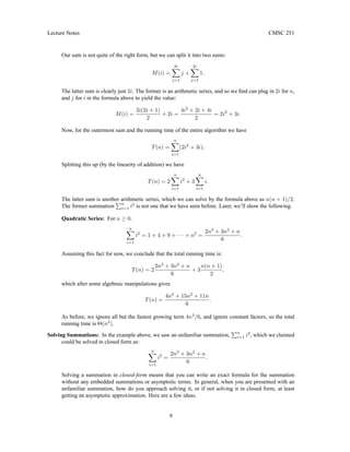
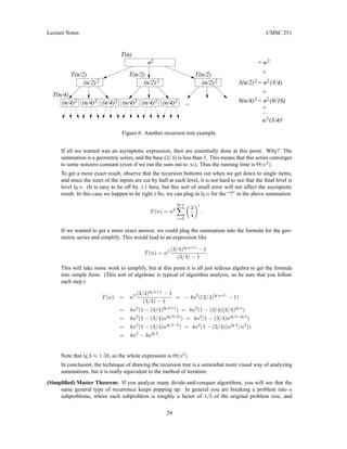
There are two principal algorithms for solving the selection problem, but they differ only in one step,
which involves judiciously choosing an item from the array, called the pivot element, which we will
denote by x. Later we will see how to choose x, but for now just think of it as a random element of A.
We then partition A into three parts. A[q] contains the element x, subarray A[p..q − 1] will contain all
the elements that are less than x, and A[q + 1..r], will contain all the element that are greater than x.
(Recall that we assumed that all the elements are distinct.) Within each subarray, the items may appear
in any order. This is illustrated below.
Before partitioing
After partitioing
2 6 4 1 3 7
9
pivot
3 5
1 9
4 6
x
p r
q
p r
A[q+1..r] x
A[p..q−1] x
5
2 7
Partition
(pivot = 4)
9
7
5
6
(k=6−4=2)
Recurse
x_rnk=2 (DONE!)
6
5
5
6
(pivot = 6)
Partition
(k=2)
Recurse
x_rnk=3
(pivot = 7)
Partition
(k=6)
Initial
x_rnk=4
6
7
3
1
4
6
2
9
5
4
1
9
5
3
7
2
6
9
5
7
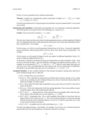
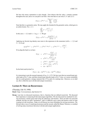
Figure 7: Selection Algorithm.
It is easy to see that the rank of the pivot x is q−p+1 in A[p..r]. Let x rnk = q −p +1. If k = x rnk,
then the pivot is the kth smallest, and we may just return it. If k x rnk, then we know that we need
to recursively search in A[p..q − 1] and if k x rnk then we need to recursively search A[q + 1..r].
In this latter case we have eliminated q smaller elements, so we want to find the element of rank k − q.
Here is the complete pseudocode.
Selection
Select(array A, int p, int r, int k) { // return kth smallest of A[p..r]
if (p == r) return A[p] // only 1 item left, return it
32](https://image.slidesharecdn.com/251-alogarithmslects-230702222135-b89653fc/85/251-Alogarithms-Lects-pdf-32-320.jpg)
![Lecture Notes CMSC 251
else {
x = Choose_Pivot(A, p, r) // choose the pivot element
q = Partition(A, p, r, x) // partition A[p..q-1], x, A[q+1..r]
x_rnk = q - p + 1 // rank of the pivot
if (k == x_rnk) return x // the pivot is the kth smallest
else if (k x_rnk)
return Select(A, p, q-1, k) // select from left subarray
else
return Select(A, q+1, r, k-x_rnk)// select from right subarray
}
}
Notice that this algorithm satisfies the basic form of a sieve algorithm. It analyzes the data (by choosing
the pivot element and partitioning) and it eliminates some part of the data set, and recurses on the rest.
When k = x rnk then we get lucky and eliminate everything. Otherwise we either eliminate the pivot
and the right subarray or the pivot and the left subarray.
We will discuss the details of choosing the pivot and partitioning later, but assume for now that they
both take Θ(n) time. The question that remains is how many elements did we succeed in eliminating?
If x is the largest or smallest element in the array, then we may only succeed in eliminating one element
with each phase. In fact, if x is one of the smallest elements of A or one of the largest, then we get
into trouble, because we may only eliminate it and the few smaller or larger elements of A. Ideally x
should have a rank that is neither too large nor too small.
Let us suppose for now (optimistically) that we are able to design the procedure Choose Pivot in
such a way that is eliminates exactly half the array with each phase, meaning that we recurse on the
remaining n/2 elements. This would lead to the following recurrence.
T(n) =
1 if n = 1,
T(n/2) + n otherwise.
We can solve this either by expansion (iteration) or the Master Theorem. If we expand this recurrence
level by level we see that we get the summation
T(n) = n +
n
2
+
n
4
+ · · · ≤
∞
X
i=0
n
2i
= n
∞
X
i=0
1
2i
.
Recall the formula for the infinite geometric series. For any c such that |c| 1,
P∞
i=0 ci
= 1/(1 − c).
Using this we have
T(n) ≤ 2n ∈ O(n).
(This only proves the upper bound on the running time, but it is easy to see that it takes at least Ω(n)
time, so the total running time is Θ(n).)
This is a bit counterintuitive. Normally you would think that in order to design a Θ(n) time algorithm
you could only make a single, or perhaps a constant number of passes over the data set. In this algorithm
we make many passes (it could be as many as lg n). However, because we eliminate a constant fraction
of elements with each phase, we get this convergent geometric series in the analysis, which shows that
the total running time is indeed linear in n. This lesson is well worth remembering. It is often possible
to achieve running times in ways that you would not expect.
Note that the assumption of eliminating half was not critical. If we eliminated even one per cent, then
the recurrence would have been T(n) = T(99n/100)+n, and we would have gotten a geometric series
involving 99/100, which is still less than 1, implying a convergent series. Eliminating any constant
fraction would have been good enough.
33](https://image.slidesharecdn.com/251-alogarithmslects-230702222135-b89653fc/85/251-Alogarithms-Lects-pdf-33-320.jpg)
![Lecture Notes CMSC 251
Choosing the Pivot: There are two issues that we have left unresolved. The first is how to choose the pivot
element, and the second is how to partition the array. Both need to be solved in Θ(n) time. The second
problem is a rather easy programming exercise. Later, when we discuss QuickSort, we will discuss
partitioning in detail.
For the rest of the lecture, let’s concentrate on how to choose the pivot. Recall that before we said that
we might think of the pivot as a random element of A. Actually this is not such a bad idea. Let’s see
why.
The key is that we want the procedure to eliminate at least some constant fraction of the array after
each partitioning step. Let’s consider the top of the recurrence, when we are given A[1..n]. Suppose
that the pivot x turns out to be of rank q in the array. The partitioning algorithm will split the array into
A[1..q − 1] x, A[q] = x and A[q + 1..n] x. If k = q, then we are done. Otherwise, we need
to search one of the two subarrays. They are of sizes q − 1 and n − q, respectively. The subarray that
contains the kth smallest element will generally depend on what k is, so in the worst case, k will be
chosen so that we have to recurse on the larger of the two subarrays. Thus if q n/2, then we may
have to recurse on the left subarray of size q − 1, and if q n/2, then we may have to recurse on the
right subarray of size n − q. In either case, we are in trouble if q is very small, or if q is very large.
If we could select q so that it is roughly of middle rank, then we will be in good shape. For example,
if n/4 ≤ q ≤ 3n/4, then the larger subarray will never be larger than 3n/4. Earlier we said that we
might think of the pivot as a random element of the array A. Actually this works pretty well in practice.
The reason is that roughly half of the elements lie between ranks n/4 and 3n/4, so picking a random
element as the pivot will succeed about half the time to eliminate at least n/4. Of course, we might be
continuously unlucky, but a careful analysis will show that the expected running time is still Θ(n). We
will return to this later.
Instead, we will describe a rather complicated method for computing a pivot element that achieves the
desired properties. Recall that we are given an array A[1..n], and we want to compute an element x
whose rank is (roughly) between n/4 and 3n/4. We will have to describe this algorithm at a very high
level, since the details are rather involved. Here is the description for Select Pivot:
Groups of 5: Partition A into groups of 5 elements, e.g. A[1..5], A[6..10], A[11..15], etc. There will
be exactly m = dn/5e such groups (the last one might have fewer than 5 elements). This can
easily be done in Θ(n) time.
Group medians: Compute the median of each group of 5. There will be m group medians. We do not
need an intelligent algorithm to do this, since each group has only a constant number of elements.
For example, we could just BubbleSort each group and take the middle element. Each will take
Θ(1) time, and repeating this dn/5e times will give a total running time of Θ(n). Copy the group
medians to a new array B.
Median of medians: Compute the median of the group medians. For this, we will have to call the
selection algorithm recursively on B, e.g. Select(B, 1, m, k), where m = dn/5e, and
k = b(m + 1)/2c. Let x be this median of medians. Return x as the desired pivot.
The algorithm is illustrated in the figure below. To establish the correctness of this procedure, we need
to argue that x satisfies the desired rank properties.
Lemma: The element x is of rank at least n/4 and at most 3n/4 in A.
Proof: We will show that x is of rank at least n/4. The other part of the proof is essentially sym-
metrical. To do this, we need to show that there are at least n/4 elements that are less than or
equal to x. This is a bit complicated, due to the floor and ceiling arithmetic, so to simplify things
we will assume that n is evenly divisible by 5. Consider the groups shown in the tabular form
above. Observe that at least half of the group medians are less than or equal to x. (Because x is
34](https://image.slidesharecdn.com/251-alogarithmslects-230702222135-b89653fc/85/251-Alogarithms-Lects-pdf-34-320.jpg)
![Lecture Notes CMSC 251
Since n/5 and 3n/4 are both less than n, we can apply the induction hypothesis, giving
T(n) ≤ c
n
5
+ c
3n
4
+ n = cn
1
5
+
3
4
+ n
= cn
19
20
+ n = n
19c
20
+ 1
.
This last expression will be ≤ cn, provided that we select c such that c ≥ (19c/20) + 1.
Solving for c we see that this is true provided that c ≥ 20.
Combining the constraints that c ≥ 1, and c ≥ 20, we see that by letting c = 20, we are done.
A natural question is why did we pick groups of 5? If you look at the proof above, you will see that it
works for any value that is strictly greater than 4. (You might try it replacing the 5 with 3, 4, or 6 and
see what happens.)
Lecture 10: Long Integer Multiplication
(Thursday, Feb 26, 1998)
Read: Todays material on integer multiplication is not covered in CLR.
Office hours: The TA, Kyongil, will have extra office hours on Monday before the midterm, from 1:00-2:00.
I’ll have office hours from 2:00-4:00 on Monday.
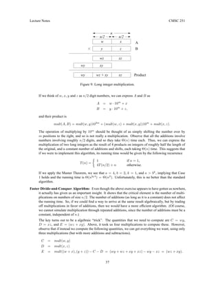
Long Integer Multiplication: The following little algorithm shows a bit more about the surprising applica-
tions of divide-and-conquer. The problem that we want to consider is how to perform arithmetic on
long integers, and multiplication in particular. The reason for doing arithmetic on long numbers stems
from cryptography. Most techniques for encryption are based on number-theoretic techniques. For
example, the character string to be encrypted is converted into a sequence of numbers, and encryption
keys are stored as long integers. Efficient encryption and decryption depends on being able to perform
arithmetic on long numbers, typically containing hundreds of digits.
Addition and subtraction on large numbers is relatively easy. If n is the number of digits, then these
algorithms run in Θ(n) time. (Go back and analyze your solution to the problem on Homework 1). But
the standard algorithm for multiplication runs in Θ(n2
) time, which can be quite costly when lots of
long multiplications are needed.
This raises the question of whether there is a more efficient way to multiply two very large numbers. It
would seem surprising if there were, since for centuries people have used the same algorithm that we
all learn in grade school. In fact, we will see that it is possible.
Divide-and-Conquer Algorithm: We know the basic grade-school algorithm for multiplication. We nor-
mally think of this algorithm as applying on a digit-by-digit basis, but if we partition an n digit number
into two “super digits” with roughly n/2 each into longer sequences, the same multiplication rule still
applies.
To avoid complicating things with floors and ceilings, let’s just assume that the number of digits n is
a power of 2. Let A and B be the two numbers to multiply. Let A[0] denote the least significant digit
and let A[n − 1] denote the most significant digit of A. Because of the way we write numbers, it is
more natural to think of the elements of A as being indexed in decreasing order from left to right as
A[n − 1..0] rather than the usual A[0..n − 1].
Let m = n/2. Let
w = A[n − 1..m] x = A[m − 1..0] and
y = B[n − 1..m] z = B[m − 1..0].
36](https://image.slidesharecdn.com/251-alogarithmslects-230702222135-b89653fc/85/251-Alogarithms-Lects-pdf-36-320.jpg)
![Lecture Notes CMSC 251
Divide-and-conquer: Understand how to design algorithms by divide-and-conquer. Understand the
divide-and-conquer algorithm for MergeSort, and be able to work an example by hand. Also
understand how the sieve technique works, and how it was used in the selection problem. (Chapt
10 on Medians; skip the randomized analysis. The material on the 2-d maxima and long integer
multiplication is not discussed in CLR.)
Lecture 11: First Midterm Exam
(Tuesday, March 3, 1998)
First midterm exam today. No lecture.
Lecture 12: Heaps and HeapSort
(Thursday, Mar 5, 1998)
Read: Chapt 7 in CLR.
Sorting: For the next series of lectures we will focus on sorting algorithms. The reasons for studying sorting
algorithms in details are twofold. First, sorting is a very important algorithmic problem. Procedures
for sorting are parts of many large software systems, either explicitly or implicitly. Thus the design of
efficient sorting algorithms is important for the overall efficiency of these systems. The other reason is
more pedagogical. There are many sorting algorithms, some slow and some fast. Some possess certain
desirable properties, and others do not. Finally sorting is one of the few problems where there provable
lower bounds on how fast you can sort. Thus, sorting forms an interesting case study in algorithm
theory.
In the sorting problem we are given an array A[1..n] of n numbers, and are asked to reorder these
elements into increasing order. More generally, A is of an array of records, and we choose one of these
records as the key value on which the elements will be sorted. The key value need not be a number. It
can be any object from a totally ordered domain. Totally ordered means that for any two elements of
the domain, x, and y, either x y, x =, or x y.
There are some domains that can be partially ordered, but not totally ordered. For example, sets can
be partially ordered under the subset relation, ⊂, but this is not a total order, it is not true that for any
two sets either x ⊂ y, x = y or x ⊃ y. There is an algorithm called topological sorting which can be
applied to “sort” partially ordered sets. We may discuss this later.
Slow Sorting Algorithms: There are a number of well-known slow sorting algorithms. These include the
following:
Bubblesort: Scan the array. Whenever two consecutive items are found that are out of order, swap
them. Repeat until all consecutive items are in order.
Insertion sort: Assume that A[1..i − 1] have already been sorted. Insert A[i] into its proper position
in this subarray, by shifting all larger elements to the right by one to make space for the new item.
Selection sort: Assume that A[1..i − 1] contain the i − 1 smallest elements in sorted order. Find the
smallest element in A[i..n], and then swap it with A[i].
These algorithms are all easy to implement, but they run in Θ(n2
) time in the worst case. We have
already seen that MergeSort sorts an array of numbers in Θ(n log n) time. We will study two others,
HeapSort and QuickSort.
39](https://image.slidesharecdn.com/251-alogarithmslects-230702222135-b89653fc/85/251-Alogarithms-Lects-pdf-39-320.jpg)
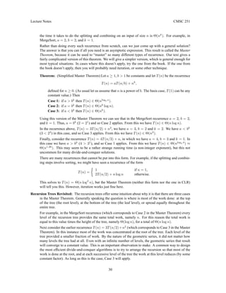
![Lecture Notes CMSC 251
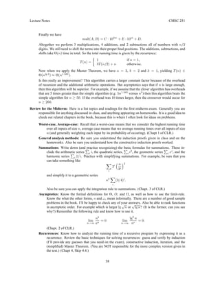
A heap is represented as an left-complete binary tree. This means that all the levels of the tree are full
except the bottommost level, which is filled from left to right. An example is shown below. The keys of
a heap are stored in something called heap order. This means that for each node u, other than the root,
key(Parent(u)) ≥ key(u). This implies that as you follow any path from a leaf to the root the keys
appear in (nonstrict) increasing order. Notice that this implies that the root is necessarily the largest
element.
4
Heap ordering
Left−complete Binary Tree
14
3
16
9
10
8 7
1
2
Figure 11: Heap.
Next time we will show how the priority queue operations are implemented for a heap.
Lecture 13: HeapSort
(Tuesday, Mar 10, 1998)
Read: Chapt 7 in CLR.
Heaps: Recall that a heap is a data structure that supports the main priority queue operations (insert and
extract max) in Θ(log n) time each. It consists of a left-complete binary tree (meaning that all levels of
the tree except possibly the bottommost) are full, and the bottommost level is filled from left to right.
As a consequence, it follows that the depth of the tree is Θ(log n) where n is the number of elements
stored in the tree. The keys of the heap are stored in the tree in what is called heap order. This means
that for each (nonroot) node its parent’s key is at least as large as its key. From this it follows that the
largest key in the heap appears at the root.
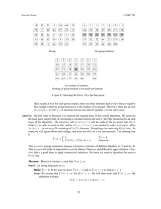
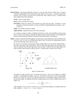
Array Storage: Last time we mentioned that one of the clever aspects of heaps is that they can be stored in
arrays, without the need for using pointers (as would normally be needed for storing binary trees). The
reason for this is the left-complete nature of the tree.
This is done by storing the heap in an array A[1..n]. Generally we will not be using all of the array,
since only a portion of the keys may be part of the current heap. For this reason, we maintain a variable
m ≤ n which keeps track of the current number of elements that are actually stored actively in the
heap. Thus the heap will consist of the elements stored in elements A[1..m].
We store the heap in the array by simply unraveling it level by level. Because the binary tree is left-
complete, we know exactly how many elements each level will supply. The root level supplies 1 node,
the next level 2, then 4, then 8, and so on. Only the bottommost level may supply fewer than the
appropriate power of 2, but then we can use the value of m to determine where the last element is. This
is illustrated below.
We should emphasize that this only works because the tree is left-complete. This cannot be used for
general trees.
41](https://image.slidesharecdn.com/251-alogarithmslects-230702222135-b89653fc/85/251-Alogarithms-Lects-pdf-41-320.jpg)
![Lecture Notes CMSC 251
3
2
1 5 6 7 8 9
4 13
12
11
10
6 7
10
16 14 10 8 7 9 4
2 1
3
n=13
m=10
Heap as an array
9
8
9
5
4
3
2
1
16
Heap as a binary tree
14
3
10
8 7
1
4
2
Figure 12: Storing a heap in an array.
We claim that to access elements of the heap involves simple arithmetic operations on the array indices.
In particular it is easy to see the following.
Left(i) : return 2i.
Right(i) : return 2i + 1.
Parent(i) : return bi/2c.
IsLeaf (i) : return Left(i) m. (That is, if i’s left child is not in the tree.)
IsRoot(i) : return i == 1.
For example, the heap ordering property can be stated as “for all i, 1 ≤ i ≤ n, if (not IsRoot(i)) then
A[Parent(i)] ≥ A[i]”.
So is a heap a binary tree or an array? The answer is that from a conceptual standpoint, it is a binary
tree. However, it is implemented (typically) as an array for space efficiency.
Maintaining the Heap Property: There is one principal operation for maintaining the heap property. It is
called Heapify. (In other books it is sometimes called sifting down.) The idea is that we are given an
element of the heap which we suspect may not be in valid heap order, but we assume that all of other
the elements in the subtree rooted at this element are in heap order. In particular this root element may
be too small. To fix this we “sift” it down the tree by swapping it with one of its children. Which child?
We should take the larger of the two children to satisfy the heap ordering property. This continues
recursively until the element is either larger than both its children or until its falls all the way to the
leaf level. Here is the pseudocode. It is given the heap in the array A, and the index i of the suspected
element, and m the current active size of the heap. The element A[max] is set to the maximum of A[i]
and it two children. If max 6= i then we swap A[i] and A[max] and then recurse on A[max].
Heapify
Heapify(array A, int i, int m) { // sift down A[i] in A[1..m]
l = Left(i) // left child
r = Right(i) // right child
max = i
if (l = m and A[l] A[max]) max = l // left child exists and larger
if (r = m and A[r] A[max]) max = r // right child exists and larger
if (max != i) { // if either child larger
swap A[i] with A[max] // swap with larger child
Heapify(A, max, m) // and recurse
}
}
42](https://image.slidesharecdn.com/251-alogarithmslects-230702222135-b89653fc/85/251-Alogarithms-Lects-pdf-42-320.jpg)
![Lecture Notes CMSC 251
See Figure 7.2 on page 143 of CLR for an example of how Heapify works (in the case where m = 10).
We show the execution on a tree, rather than on the array representation, since this is the most natural
way to conceptualize the heap. You might try simulating this same algorithm on the array, to see how
it works at a finer details.
Note that the recursive implementation of Heapify is not the most efficient. We have done so because
many algorithms on trees are most naturally implemented using recursion, so it is nice to practice this
here. It is possible to write the procedure iteratively. This is left as an exercise.
The HeapSort algorithm will consist of two major parts. First building a heap, and then extracting the
maximum elements from the heap, one by one. We will see how to use Heapify to help us do both of
these.
How long does Hepify take to run? Observe that we perform a constant amount of work at each level
of the tree until we make a call to Heapify at the next lower level of the tree. Thus we do O(1) work
for each level of the tree which we visit. Since there are Θ(log n) levels altogether in the tree, the total
time for Heapify is O(log n). (It is not Θ(log n) since, for example, if we call Heapify on a leaf, then
it will terminate in Θ(1) time.)
Building a Heap: We can use Heapify to build a heap as follows. First we start with a heap in which the
elements are not in heap order. They are just in the same order that they were given to us in the array
A. We build the heap by starting at the leaf level and then invoke Heapify on each node. (Note: We
cannot start at the top of the tree. Why not? Because the precondition which Heapify assumes is that
the entire tree rooted at node i is already in heap order, except for i.) Actually, we can be a bit more
efficient. Since we know that each leaf is already in heap order, we may as well skip the leaves and
start with the first nonleaf node. This will be in position bn/2c. (Can you see why?)
Here is the code. Since we will work with the entire array, the parameter m for Heapify, which indicates
the current heap size will be equal to n, the size of array A, in all the calls.
BuildHeap
BuildHeap(int n, array A[1..n]) { // build heap from A[1..n]
for i = n/2 downto 1 {
Heapify(A, i, n)
}
}
An example of BuildHeap is shown in Figure 7.3 on page 146 of CLR. Since each call to Heapify
takes O(log n) time, and we make roughly n/2 calls to it, the total running time is O((n/2) log n) =
O(n log n). Next time we will show that this actually runs faster, and in fact it runs in Θ(n) time.
HeapSort: We can now give the HeapSort algorithm. The idea is that we need to repeatedly extract the
maximum item from the heap. As we mentioned earlier, this element is at the root of the heap. But
once we remove it we are left with a hole in the tree. To fix this we will replace it with the last leaf in
the tree (the one at position A[m]). But now the heap order will very likely be destroyed. So we will
just apply Heapify to the root to fix everything back up.
HeapSort
HeapSort(int n, array A[1..n]) { // sort A[1..n]
BuildHeap(n, A) // build the heap
m = n // initially heap contains all
while (m = 2) {
swap A[1] with A[m] // extract the m-th largest
m = m-1 // unlink A[m] from heap
43](https://image.slidesharecdn.com/251-alogarithmslects-230702222135-b89653fc/85/251-Alogarithms-Lects-pdf-43-320.jpg)
![Lecture Notes CMSC 251
It is worthwhile pausing here a moment. This is the second time we have seen a relatively complex
structured algorithm, with doubly nested loops, come out with a running time of Θ(n). (The other
example was the median algorithm, based on the sieve technique. Actually if you think deeply about
this, there is a sense in which a parallel version of BuildHeap can be viewed as operating like a sieve,
but maybe this is getting too philosophical.) Perhaps a more intuitive way to describe what is happening
here is to observe an important fact about binary trees. This is that the vast majority of nodes are at the
lowest level of the tree. For example, in a complete binary tree of height h there is a total of n ≈ 2h+1
nodes in total, and the number of nodes in the bottom 3 levels alone is
2h
+ 2h−1
+ 2h−2
=
n
2
+
n
4
+
n
8
=
7n
8
= 0.875n.
That is, almost 90% of the nodes of a complete binary tree reside in the 3 lowest levels. Thus the lesson
to be learned is that when designing algorithms that operate on trees, it is important to be most efficient
on the bottommost levels of the tree (as BuildHeap is) since that is where most of the weight of the tree
resides.
Partitioning: Our next sorting algorithm is QuickSort. QuickSort is interesting in a number of respects.
First off, (as we will present it) it is a randomized algorithm, which means that it makes use of a ran-
dom number generator. We will show that in the worst case its running time is O(n2
), its expected
case running time is O(n log n). Moreover, this expected case running time occurs with high proba-
bility, in that the probability that the algorithm takes significantly more than O(n log n) time is rapidly
decreasing function of n. In addition, QuickSort has a better locality-of-reference behavior than either
MergeSort or HeapSort, and thus it tends to run fastest of all three algorithms. This is how it got its
name. QuickSort (and its variants) are considered the methods of choice for most standard library
sorting algorithms.
Next time we will discuss QuickSort. Today we will discuss one aspect of QuickSort, namely the
partitioning algorithm. This is the same partitioning algorithm which we discussed when we talked
about the selection (median) problem. We are given an array A[p..r], and a pivot element x chosen
from the array. Recall that the partitioning algorithm is suppose to partition A into three subarrays:
A[p..q − 1] whose elements are all less than or equal to x, A[q] = x, and A[q + 1..r] whose elements
are greater than or equal to x. We will assume that x is the first element of the subarray, that is,
x = A[p]. If a different rule is used for selecting x, this is easily handled by swapping this element
with A[p] before calling this procedure.
We will present a different algorithm from the one given in the text (in Section 8.1). This algorithm is
a little easier to verify the correctness, and a little easier to analyze. (But I suspect that the one in the
text is probably a bit for efficient for actual implementation.)
This algorithm works by maintaining the following invariant condition. The subarray is broken into
four segments. The boundaries between these items are indicated by the indices p, q, s, and r.
(1) A[p] = x is the pivot value,
(2) A[p + 1..q] contains items that are less than x,
(3) A[q + 1..s − 1] contains items that are greater than or equal to x, and
(4) A[s..r] contains items whose values are currently unknown.
This is illustrated below.
The algorithm begins by setting q = p and s = p + 1. With each step through the algorithm we test the
value of A[s] against x. If A[s] ≥ x, then we can simply increment s. Otherwise we increment q, swap
A[s] with A[q], and then increment s. Notice that in either case, the invariant is still maintained. In the
first case this is obvious. In the second case, A[q] now holds a value that is less than x, and A[s − 1]
now holds a value that is greater than or equal to x. The algorithm ends when s = r, meaning that
46](https://image.slidesharecdn.com/251-alogarithmslects-230702222135-b89653fc/85/251-Alogarithms-Lects-pdf-46-320.jpg)
![Lecture Notes CMSC 251
configuration
p r
q s
x ?
p r
q s
= x
x
q
swap
x
Initial configuration
Final configuration
Intermediate
x x = x ?
Figure 14: Partitioning intermediate structure.
all of the elements have been processed. To finish things off we swap A[p] (the pivot) with A[q], and
return the value of q. Here is the complete code:
Partition
Partition(int p, int r, array A) { // 3-way partition of A[p..r]
x = A[p] // pivot item in A[p]
q = p
for s = p+1 to r do {
if (A[s] x) {
q = q+1
swap A[q] with A[s]
}
}
swap A[p] with A[q] // put the pivot into final position
return q // return location of pivot
}
An example is shown below.
Lecture 15: QuickSort
(Tuesday, Mar 17, 1998)
Revised: March 18. Fixed a bug in the analysis.
Read: Chapt 8 in CLR. My presentation and analysis are somewhat different than the text’s.
QuickSort and Randomized Algorithms: Early in the semester we discussed the fact that we usually study
the worst-case running times of algorithms, but sometimes average-case is a more meaningful measure.
Today we will study QuickSort. It is a worst-case Θ(n2
) algorithm, whose expected-case running time
is Θ(n log n).
We will present QuickSort as a randomized algorithm, that is, an algorithm which makes random
choices. There are two common types of randomized algorithms:
Monte Carlo algorithms: These algorithms may produce the wrong result, but the probability of this
occurring can be made arbitrarily small by the user. Usually the lower you make this probability,
the longer the algorithm takes to run.
47](https://image.slidesharecdn.com/251-alogarithmslects-230702222135-b89653fc/85/251-Alogarithms-Lects-pdf-47-320.jpg)
![Lecture Notes CMSC 251
Final swap
3
7 1
q
8
4
s
5 3 7
3
6
s
4 8
q
1
7 3
6
5 3
3
1
5 3 7 1
8
4
s
q
6
3
5
4 6
q
8
1
s
3 7
4 6
3
q
8
p r
5 3 8 6 4 3
q s
1
7
5 3 8 6 4 3
q
7 1
s
5 3 8 6 4 3
q
7 1
s
5
5 3 8 6 4 3
s
q
7 1
Figure 15: Partitioning example.
Las Vegas algorithms: These algorithms always produce the correct result, but the running time is a
random variable. In these cases the expected running time, averaged over all possible random
choices is the measure of the algorithm’s running time.
The most well known Monte Carlo algorithm is one for determining whether a number is prime. This
is an important problem in cryptography. The QuickSort algorithm that we will discuss today is an ex-
ample of a Las Vegas algorithm. Note that QuickSort does not need to be implemented as a randomized
algorithm, but as we shall see, this is generally considered the safest implementation.
QuickSort Overview: QuickSort is also based on the divide-and-conquer design paradigm. Unlike Merge-
Sort where most of the work is done after the recursive call returns, in QuickSort the work is done
before the recursive call is made. Here is an overview of QuickSort. Note the similarity with the selec-
tion algorithm, which we discussed earlier. Let A[p..r] be the (sub)array to be sorted. The initial call
is to A[1..n].
Basis: If the list contains 0 or 1 elements, then return.
Select pivot: Select a random element x from the array, called the pivot.
Partition: Partition the array in three subarrays, those elements A[1..q − 1] ≤ x, A[q] = x, and
A[q + 1..n] ≥ x.
Recurse: Recursively sort A[1..q − 1] and A[q + 1..n].
The pseudocode for QuickSort is given below. The initial call is QuickSort(1, n, A). The Partition
routine was discussed last time. Recall that Partition assumes that the pivot is stored in the first element
of A. Since we want a random pivot, we pick a random index i from p to r, and then swap A[i] with
A[p].
QuickSort
QuickSort(int p, int r, array A) { // Sort A[p..r]
if (r = p) return // 0 or 1 items, return
i = a random index from [p..r] // pick a random element
48](https://image.slidesharecdn.com/251-alogarithmslects-230702222135-b89653fc/85/251-Alogarithms-Lects-pdf-48-320.jpg)
![Lecture Notes CMSC 251
swap A[i] with A[p] // swap pivot into A[p]
q = Partition(p, r, A) // partition A about pivot
QuickSort(p, q-1, A) // sort A[p..q-1]
QuickSort(q+1, r, A) // sort A[q+1..r]
}
QuickSort Analysis: The correctness of QuickSort should be pretty obvious. However its analysis is not
so obvious. It turns out that the running time of QuickSort depends heavily on how good a job we
do in selecting the pivot. In particular, if the rank of the pivot (recall that this means its position in
the final sorted list) is very large or very small, then the partition will be unbalanced. We will see that
unbalanced partitions (like unbalanced binary trees) are bad, and result is poor running times. However,
if the rank of the pivot is anywhere near the middle portion of the array, then the split will be reasonably
well balanced, and the overall running time will be good. Since the pivot is chosen at random by our
algorithm, we may do well most of the time and poorly occasionally. We will see that the expected
running time is O(n log n).
Worst-case Analysis: Let’s begin by considering the worst-case performance, because it is easier than the
average case. Since this is a recursive program, it is natural to use a recurrence to describe its running
time. But unlike MergeSort, where we had control over the sizes of the recursive calls, here we do
not. It depends on how the pivot is chosen. Suppose that we are sorting an array of size n, A[1..n],
and further suppose that the pivot that we select is of rank q, for some q in the range 1 to n. It takes
Θ(n) time to do the partitioning and other overhead, and we make two recursive calls. The first is to
the subarray A[1..q − 1] which has q − 1 elements, and the other is to the subarray A[q + 1..n] which
has r − (q + 1) + 1 = r − q elements. So if we ignore the Θ (as usual) we get the recurrence:
T(n) = T(q − 1) + T(n − q) + n.
This depends on the value of q. To get the worst case, we maximize over all possible values of q. As a
basis we have that T(0) = T(1) = Θ(1). Putting this together we have
T(n) =
1 if n ≤ 1
max1≤q≤n(T(q − 1) + T(n − q) + n) otherwise.
Recurrences that have max’s and min’s embedded in them are very messy to solve. The key is deter-
mining which value of q gives the maximum. (A rule of thumb of algorithm analysis is that the worst
cases tends to happen either at the extremes or in the middle. So I would plug in the value q = 1, q = n,
and q = n/2 and work each out.) In this case, the worst case happens at either of the extremes (but see
the book for a more careful analysis based on an analysis of the second derivative). If we expand the
recurrence in the case q = 1 we get:
T(n) ≤ T(0) + T(n − 1) + n = 1 + T(n − 1) + n
= T(n − 1) + (n + 1)
= T(n − 2) + n + (n + 1)
= T(n − 3) + (n − 1) + n + (n + 1)
= T(n − 4) + (n − 2) + (n − 1) + n + (n + 1)
= . . .
= T(n − k) +
k−2
X
i=−1
(n − i).
49](https://image.slidesharecdn.com/251-alogarithmslects-230702222135-b89653fc/85/251-Alogarithms-Lects-pdf-49-320.jpg)
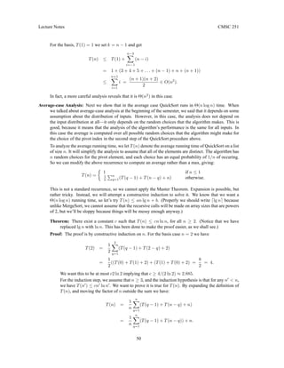
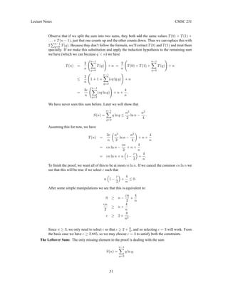
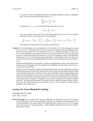
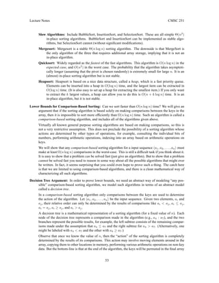
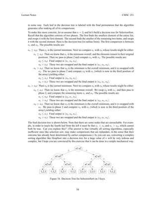
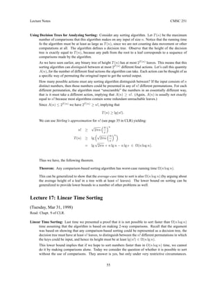
![Lecture Notes CMSC 251
Many applications involve sorting small integers (e.g. sorting characters, exam scores, last four digits
of a social security number, etc.). We present three algorithms based on the theme of speeding up
sorting in special cases, by not making comparisons.
Counting Sort: Counting sort assumes that each input is an integer in the range from 1 to k. The algorithm
sorts in Θ(n + k) time. If k is known to be Θ(n), then this implies that the resulting sorting algorithm
is Θ(n) time.
The basic idea is to determine, for each element in the input array, its rank in the final sorted array.
Recall that the rank of a item is the number of elements in the array that are less than or equal to it.
Notice that once you know the rank of every element, you sort by simply copying each element to the
appropriate location of the final sorted output array. The question is how to find the rank of an element
without comparing it to the other elements of the array? Counting sort uses the following three arrays.
As usual A[1..n] is the input array. Recall that although we usually think of A as just being a list of
numbers, it is actually a list of records, and the numeric value is the key on which the list is being
sorted. In this algorithm we will be a little more careful to distinguish the entire record A[j] from the
key A[j].key.
We use three arrays:
A[1..n] : Holds the initial input. A[j] is a record. A[j].key is the integer key value on which to sort.
B[1..n] : Array of records which holds the sorted output.
R[1..k] : An array of integers. R[x] is the rank of x in A, where x ∈ [1..k].
The algorithm is remarkably simple, but deceptively clever. The algorithm operates by first construct-
ing R. We do this in two steps. First we set R[x] to be the number of elements of A[j] whose key
is equal to x. We can do this initializing R to zero, and then for each j, from 1 to n, we increment
R[A[j].key] by 1. Thus, if A[j].key = 5, then the 5th element of R is incremented, indicating that we
have seen one more 5. To determine the number of elements that are less than or equal to x, we replace
R[x] with the sum of elements in the subarray R[1..x]. This is done by just keeping a running total of
the elements of R.
Now R[x] now contains the rank of x. This means that if x = A[j].key then the final position of A[j]
should be at position R[x] in the final sorted array. Thus, we set B[R[x]] = A[j]. Notice that this
copies the entire record, not just the key value. There is a subtlety here however. We need to be careful
if there are duplicates, since we do not want them to overwrite the same location of B. To do this, we
decrement R[i] after copying.
Counting Sort
CountingSort(int n, int k, array A, array B) { // sort A[1..n] to B[1..n]
for x = 1 to k do R[x] = 0 // initialize R
for j = 1 to n do R[A[j].key]++ // R[x] = #(A[j] == x)
for x = 2 to k do R[x] += R[x-1] // R[x] = rank of x
for j = n downto 1 do { // move each element of A to B
x = A[j].key // x = key value
B[R[x]] = A[j] // R[x] is where to put it
R[x]-- // leave space for duplicates
}
}
There are four (unnested) loops, executed k times, n times, k − 1 times, and n times, respectively,
so the total running time is Θ(n + k) time. If k = O(n), then the total running time is Θ(n). The
figure below shows an example of the algorithm. You should trace through a few examples, to convince
yourself how it works.
56](https://image.slidesharecdn.com/251-alogarithmslects-230702222135-b89653fc/85/251-Alogarithms-Lects-pdf-56-320.jpg)
![Lecture Notes CMSC 251
s
s
r
r
r
e
e
a
4
3
2
1 5
4
3
2
1
5
4
2
2
s
3
1 3
3
3
1
4
3
3
1
4
3
3
1
1
v
v
v
v
v
s
5
1
4
3
2
1 5
A R R
R
R
R
R
R
B
B
B
B
B
Key
Other data
2
3
2
2
5
3
2
1
5
2
2
1
4
2
2
1
4
2
2
0
4
3
e
1
2
0
2
3
1
3
4
1
a s v
r
Figure 17: Counting Sort.
Obviously this not an in-place sorting algorithm (we need two additional arrays). However it is a stable
sorting algorithm. I’ll leave it as an exercise to prove this. (As a hint, notice that the last loop runs
down from n to 1. It would not be stable if the loop were running the other way.)
Radix Sort: The main shortcoming of counting sort is that it is only really (due to space requirements) for
small integers. If the integers are in the range from 1 to 1 million, we may not want to allocate an
array of a million elements. Radix sort provides a nice way around this by sorting numbers one digit
at a time. Actually, what constitutes a “digit” is up to the implementor. For example, it is typically
more convenient to sort by bytes rather than digits (especially for sorting character strings). There is a
tradeoff between the space and time.
The idea is very simple. Let’s think of our list as being composed of n numbers, each having d decimal
digits (or digits in any base). Let’s suppose that we have access to a stable sorting algorithm, like
Counting Sort. To sort these numbers we can simply sort repeatedly, starting at the lowest order digit,
and finishing with the highest order digit. Since the sorting algorithm is stable, we know that if the
numbers are already sorted with respect to low order digits, and then later we sort with respect to high
order digits, numbers having the same high order digit will remain sorted with respect to their low
order digit. As usual, let A[1..n] be the array to sort, and let d denote the number of digits in A. We
will not discuss how it is that A is broken into digits, but this might be done through bit manipulations
(shifting and masking off bits) or by accessing elements byte-by-byte, etc.
Radix Sort
RadixSort(int n, int d, array A) { // sort A[1..n] with d digits
for i = 1 to d do {
Sort A (stably) with respect to i-th lowest order digit;
}
}
57](https://image.slidesharecdn.com/251-alogarithmslects-230702222135-b89653fc/85/251-Alogarithms-Lects-pdf-57-320.jpg)
![Lecture Notes CMSC 251
Here is an example.
576 49[4] 9[5]4 [1]76 176
494 19[4] 5[7]6 [1]94 194
194 95[4] 1[7]6 [2]78 278
296 =⇒ 57[6] =⇒ 2[7]8 =⇒ [2]96 =⇒ 296
278 29[6] 4[9]4 [4]94 494
176 17[6] 1[9]4 [5]76 576
954 27[8] 2[9]6 [9]54 954
The running time is clearly Θ(d(n + k)) where d is the number of digits, n is the length of the list, and
k is the number of values a digit can have. This is usually a constant, but the algorithm’s running time
will be Θ(dn) as long as k ∈ O(n).
Notice that we can be quite flexible in the definition of what a “digit” is. It can be any number in the
range from 1 to cn for some constant c, and we will still have an Θ(n) time algorithm. For example,
if we have d = 2 and set k = n, then we can sort numbers in the range n ∗ n = n2
in Θ(n) time. In
general, this can be used to sort numbers in the range from 1 to nd
in Θ(dn) time.
At this point you might ask, since a computer integer word typically consists of 32 bits (4 bytes), then
doesn’t this imply that we can sort any array of integers in O(n) time (by applying radix sort on each
of the d = 4 bytes)? The answer is yes, subject to this word-length restriction. But you should be
careful about attempting to make generalizations when the sizes of the numbers are not bounded. For
example, suppose you have n keys and there are no duplicate values. Then it follows that you need
at least B = dlg ne bits to store these values. The number of bytes is d = dB/8e. Thus, if you were
to apply radix sort in this situation, the running time would be Θ(dn) = Θ(n log n). So there is no
real asymptotic savings here. Furthermore, the locality of reference behavior of Counting Sort (and
hence of RadixSort) is not as good as QuickSort. Thus, it is not clear whether it is really faster to use
RadixSort over QuickSort. This is at a level of similarity, where it would probably be best to implement
both algorithms on your particular machine to determine which is really faster.
Lecture 18: Review for Second Midterm
(Thursday, Apr 2, 1998)
General Remarks: Up to now we have covered the basic techniques for analyzing algorithms (asymptotics,
summations, recurrences, induction), have discussed some algorithm design techniques (divide-and-
conquer in particular), and have discussed sorting algorithm and related topics. Recall that our goal is
to provide you with the necessary tools for designing and analyzing efficient algorithms.
Material from Text: You are only responsible for material that has been covered in class or on class assign-
ments. However it is always a good idea to see the text to get a better insight into some of the topics
we have covered. The relevant sections of the text are the following.
• Review Chapts 1: InsertionSort and MergeSort.
• Chapt 7: Heaps, HeapSort. Look at Section 7.5 on priority queues, even though we didn’t cover
it in class.
• Chapt 8: QuickSort. You are responsible for the partitioning algorithm which we gave in class,
not the one in the text. Section 8.2 gives some good intuition on the analysis of QuickSort.
• Chapt 9 (skip 9.4): Lower bounds on sorting, CountingSort, RadixSort.
58](https://image.slidesharecdn.com/251-alogarithmslects-230702222135-b89653fc/85/251-Alogarithms-Lects-pdf-58-320.jpg)
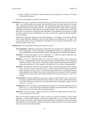
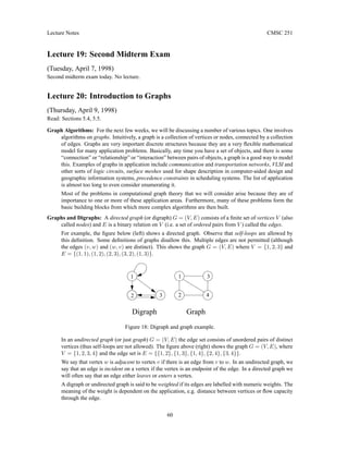
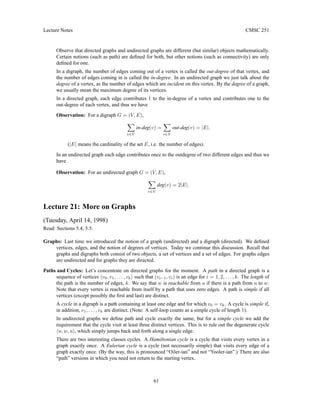
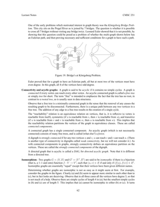
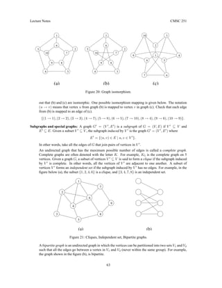
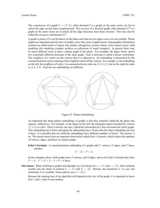
![Lecture Notes CMSC 251
Observation: For a digraph e ≤ n2
= O(n2
). For an undirected graph e ≤ n
2
= n(n − 1)/2 =
O(n2
).
A graph or digraph is allowed to have no edges at all. One interesting question is what the minimum
number of edges that a connected graph must have.
We say that a graph is sparse if e is much less than n2
.
For example, the important class of planar graphs (graphs which can be drawn on the plane so that no
two edges cross over one another) e = O(n). In most application areas, very large graphs tend to be
sparse. This is important to keep in mind when designing graph algorithms, because when n is really
large and O(n2
) running time is often unacceptably large for real-time response.
Lecture 22: Graphs Representations and BFS
(Thursday, April 16, 1998)
Read: Sections 23.1 through 23.3 in CLR.
Representations of Graphs and Digraphs: We will describe two ways of representing graphs and digraphs.
First we show how to represent digraphs. Let G = (V, E) be a digraph with n = |V | and let e = |E|.
We will assume that the vertices of G are indexed {1, 2, . . . , n}.
Adjacency Matrix: An n × n matrix defined for 1 ≤ v, w ≤ n.
A[v, w] =
1 if (v, w) ∈ E
0 otherwise.
If the digraph has weights we can store the weights in the matrix. For example if (v, w) ∈ E then
A[v, w] = W(v, w) (the weight on edge (v, w)). If (v, w) /
∈ E then generally W(v, w) need
not be defined, but often we set it to some “special” value, e.g. A(v, w) = −1, or ∞. (By ∞
we mean (in practice) some number which is larger than any allowable weight. In practice, this
might be some machine dependent constant like MAXINT.)
Adjacency List: An array Adj[1 . . . n] of pointers where for 1 ≤ v ≤ n, Adj[v] points to a linked list
containing the vertices which are adjacent to v (i.e. the vertices that can be reached from v by a
single edge). If the edges have weights then these weights may also be stored in the linked list
elements.
3
1
1
0
1
0
1
1
0
0
2 3
1
2
3
2
1
Adjacency matrix
Adj
Adjacency list
3
2
2
3
1
3
2
1
1
Figure 23: Adjacency matrix and adjacency list for digraphs.
We can represent undirected graphs using exactly the same representation, but we will store each edge
twice. In particular, we representing the undirected edge {v, w} by the two oppositely directed edges
(v, w) and (w, v). Notice that even though we represent undirected graphs in the same way that we
65](https://image.slidesharecdn.com/251-alogarithmslects-230702222135-b89653fc/85/251-Alogarithms-Lects-pdf-65-320.jpg)
![Lecture Notes CMSC 251
represent digraphs, it is important to remember that these two classes of objects are mathematically
distinct from one another.
This can cause some complications. For example, suppose you write an algorithm that operates by
marking edges of a graph. You need to be careful when you mark edge (v, w) in the representation
that you also mark (w, v), since they are both the same edge in reality. When dealing with adjacency
lists, it may not be convenient to walk down the entire linked list, so it is common to include cross links
between corresponding edges.
2
1
1 2 3
1
1
0
1
0
1
3
Adjacency list (with crosslinks)
Adjacency matrix
Adj
4
1
1 2 4
4
2
3
1
3
4
1
1
1
0
0
0
1
1
1 0
4
3
2
1
3
1
3
2
4
Figure 24: Adjacency matrix and adjacency list for graphs.
An adjacency matrix requires Θ(n2
) storage and an adjacency list requires Θ(n+e) storage (one entry
for each vertex in Adj and each list has outdeg(v) entries, which when summed is Θ(e). For sparse
graphs the adjacency list representation is more cost effective.
Shortest Paths: To motivate our first algorithm on graphs, consider the following problem. You are given
an undirected graph G = (V, E) (by the way, everything we will be saying can be extended to directed
graphs, with only a few small changes) and a source vertex s ∈ V . The length of a path in a graph
(without edge weights) is the number of edges on the path. We would like to find the shortest path from
s to each other vertex in G. If there are ties (two shortest paths of the same length) then either path
may be chosen arbitrarily.
The final result will be represented in the following way. For each vertex v ∈ V , we will store d[v]
which is the distance (length of the shortest path) from s to v. Note that d[s] = 0. We will also store a
predecessor (or parent) pointer π[v], which indicates the first vertex along the shortest path if we walk
from v backwards to s. We will let π[s] = NIL.
It may not be obvious at first, but these single predecessor pointers are sufficient to reconstruct the
shortest path to any vertex. Why? We make use of a simple fact which is an example of a more general
principal of many optimization problems, called the principal of optimality. For a path to be a shortest
path, every subpath of the path must be a shortest path. (If not, then the subpath could be replaced with
a shorter subpath, implying that the original path was not shortest after all.)
Using this observation, we know that the last edge on the shortest path from s to v is the edge (u, v),
then the first part of the path must consist of a shortest path from s to u. Thus by following the
predecessor pointers we will construct the reverse of the shortest path from s to v.
Obviously, there is simple brute-force strategy for computing shortest paths. We could simply start
enumerating all simple paths starting at s, and keep track of the shortest path arriving at each vertex.
However, since there can be as many as n! simple paths in a graph (consider a complete graph), then
this strategy is clearly impractical.
Here is a simple strategy that is more efficient. Start with the source vertex s. Clearly, the distance to
each of s’s neighbors is exactly 1. Label all of them with this distance. Now consider the unvisited
66](https://image.slidesharecdn.com/251-alogarithmslects-230702222135-b89653fc/85/251-Alogarithms-Lects-pdf-66-320.jpg)
![Lecture Notes CMSC 251
2
2
2
2
2
2
3
3
3
3
3
s
1
1
1
s
s
: Finished
: Discovered
: Undiscovered
Figure 25: Breadth-first search for shortest paths.
neighbors of these neighbors. They will be at distance 2 from s. Next consider the unvisited neighbors
of the neighbors of the neighbors, and so on. Repeat this until there are no more unvisited neighbors left
to visit. This algorithm can be visualized as simulating a wave propagating outwards from s, visiting
the vertices in bands at ever increasing distances from s.
Breadth-first search: Given an graph G = (V, E), breadth-first search starts at some source vertex s and
“discovers” which vertices are reachable from s. Define the distance between a vertex v and s to be the
minimum number of edges on a path from s to v. Breadth-first search discovers vertices in increasing
order of distance, and hence can be used as an algorithm for computing shortest paths. At any given
time there is a “frontier” of vertices that have been discovered, but not yet processed. Breadth-first
search is named because it visits vertices across the entire “breadth” of this frontier.
Initially all vertices (except the source) are colored white, meaning that they have not been seen. When
a vertex has first been discovered, it is colored gray (and is part of the frontier). When a gray vertex is
processed, then it becomes black.
Breadth-First Search
BFS(graph G=(V,E), vertex s) {
int d[1..size(V)] // vertex distances
int color[1..size(V)] // vertex colors
vertex pred[1..size(V)] // predecessor pointers
queue Q = empty // FIFO queue
for each u in V { // initialization
color[u] = white
d[u] = INFINITY
pred[u] = NULL
}
color[s] = gray // initialize source s
d[s] = 0
enqueue(Q, s) // put source in the queue
while (Q is nonempty) {
u = dequeue(Q) // u is the next vertex to visit
for each v in Adj[u] {
if (color[v] == white) { // if neighbor v undiscovered
color[v] = gray // ...mark it discovered
d[v] = d[u]+1 // ...set its distance
pred[v] = u // ...and its predecessor
67](https://image.slidesharecdn.com/251-alogarithmslects-230702222135-b89653fc/85/251-Alogarithms-Lects-pdf-67-320.jpg)
![Lecture Notes CMSC 251
enqueue(Q, v) // ...put it in the queue
}
}
color[u] = black // we are done with u
}
}
The search makes use of a queue, a first-in first-out list, where elements are removed in the same order
they are inserted. The first item in the queue (the next to be removed) is called the head of the queue.
We will also maintain arrays color[u] which holds the color of vertex u (either white, gray or black),
pred[u] which points to the predecessor of u (i.e. the vertex who first discovered u, and d[u], the
distance from s to u. Only the color is really needed for the search, but the others are useful depending
on the application.
s
t
u v
Q: x, u, w
s
t
u v w
x
Q: w, t
s
t
u v w
x
Q: u, w
Q: v, x
w
x
s
t
u v w
x s
t
u v w
x
Q: s
t
u v w
x
s
Q: t
?
?
?
1
0 1
?
2
2
1
1
0
2 2
1
0
1
1
3
2
?
?
?
?
? 0
0
1
1
3
2 2
2
? 0 1
Figure 26: Breadth-first search: Example.
Observe that the predecessor pointers of the BFS search define an inverted tree. If we reverse these
edges we get a rooted unordered tree called a BFS tree for G. (Note that there are many potential BFS
trees for a given graph, depending on where the search starts, and in what order vertices are placed on
the queue.) These edges of G are called tree edges and the remaining edges of G are called cross edges.
It is not hard to prove that if G is an undirected graph, then cross edges always go between two nodes
that are at most one level apart in the BFS tree. The reason is that if any cross edge spanned two or
more levels, then when the vertex at the higher level (closer to the root) was being processed, it would
have discovered the other vertex, implying that the other vertex would appear on the very next level of
the tree, a contradiction. (In a directed graph cross edges will generally go down at most 1 level, but
they may come up an arbitrary number of levels.)
Analysis: The running time analysis of BFS is similar to the running time analysis of many graph traversal
algorithms. Let n = |V | and e = |E|. Observe that the initialization portion requires Θ(n) time.
The real meat is in the traversal loop. Since we never visit a vertex twice, the number of times we go
through the while loop is at most n (exactly n assuming each vertex is reachable from the source). The
number of iterations through the inner for loop is proportional to deg(u) + 1. (The +1 is because even
if deg(u) = 0, we need to spend a constant amount of time to set up the loop.) Summing up over all
vertices we have the running time
T(n) = n +
X
u∈V
(deg(u) + 1) = n +
X
u∈V
deg(u) + n = 2n + 2e ∈ Θ(n + e).
68](https://image.slidesharecdn.com/251-alogarithmslects-230702222135-b89653fc/85/251-Alogarithms-Lects-pdf-68-320.jpg)
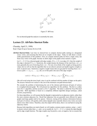
![Lecture Notes CMSC 251
there are no cycles whose total weight is negative. It is easy to see why this causes problems. If the
shortest path ever enters such a cycle, it would never exit. Why? Because by going round the cycle
over and over, the cost will become smaller and smaller. Thus, the shortest path would have a weight
of −∞, and would consist of an infinite number of edges. Disallowing negative weight cycles will rule
out the possibility this absurd situation.
Input Format: The input is an n × n matrix W of edge weights, which are based on the edge weights in the
digraph. We let wij denote the entry in row i and column j of W.
wij =
0 if i = j,
W(i, j) if i 6= j and (i, j) ∈ E,
+∞ if i 6= j and (i, j) /
∈ E.
Setting wij = ∞ if there is no edge, intuitively means that there is no direct link between these two
nodes, and hence the direct cost is infinite. The reason for setting wii = 0 is that intuitively the cost
of getting from any vertex to should be 0, since we have no distance to travel. Note that in digraphs
it is possible to have self-loop edges, and so W(i, j) may generally be nonzero. Notice that it cannot
be negative (otherwise we would have a negative cost cycle consisting of this single edge). If it is
positive, then it never does us any good to follow this edge (since it increases our cost and doesn’t take
us anywhere new).
The output will be an n × n distance matrix D = dij where dij = δ(i, j), the shortest path cost from
vertex i to j. Recovering the shortest paths will also be an issue. To help us do this, we will also
compute an auxiliary matrix pred[i, j]. The value of pred[i, j] will be a vertex that is somewhere along
the shortest path from i to j. If the shortest path travels directly from i to j without passing through
any other vertices, then pred[i, j] will be set to null. We will see later than using these values it will be
possible to reconstruct any shortest path in Θ(n) time.
Dynamic Programming for Shortest Paths: The algorithm is based on a technique called dynamic pro-
gramming. Dynamic programming problems are typically optimization problems (find the smallest or
largest solution, subject to various constraints). The technique is related to divide-and-conquer, in the
sense that it breaks problems down into smaller problems that it solves recursively. However, because
of the somewhat different nature of dynamic programming problems, standard divide-and-conquer
solutions are not usually efficient. The basic elements that characterize a dynamic programming algo-
rithm are:
Substructure: Decompose the problem into smaller subproblems.
Optimal substructure: Each of the subproblems should be solved optimally.
Bottom-up computation: Combine solutions on small subproblems to solve larger subproblems, and
eventually to arrive at a solution to the complete problem.
The question is how to decompose the shortest path problem into subproblems in a meaningful way.
There is one very natural way to do this. What is remarkable, is that this does not lead to the best solu-
tion. First we will introduce the natural decomposition, and later present the Floyd-Warshall algorithm
makes use of a different, but more efficient dynamic programming formulation.
Path Length Formulation: We will concentrate just on computing the cost of the shortest path, not the path
itself. Let us first sketch the natural way to break the problem into subproblems. We want to find some
parameter, which constrains the estimates to the shortest path costs. At first the estimates will be crude.
As this parameter grows, the shortest paths cost estimates should converge to their correct values. A
natural way to do this is to restrict the number of edges that are allowed to be in the shortest path.
For 0 ≤ m ≤ n − 1, define d
(m)
ij to be the cost of the shortest path from vertex i to vertex j that
contains at most m edges. Let D(m)
denote the matrix whose entries are these values. The idea is to
70](https://image.slidesharecdn.com/251-alogarithmslects-230702222135-b89653fc/85/251-Alogarithms-Lects-pdf-70-320.jpg)
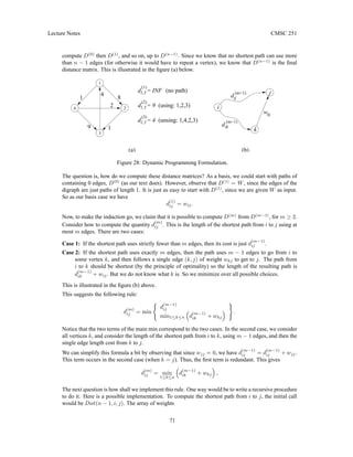
![Lecture Notes CMSC 251
Recursive Shortest Paths
Dist(int m, int i, int j) {
if (m == 1) return W[i,j] // single edge case
best = INF
for k = 1 to n do
best = min(best, Dist(m-1, i, k) + w[k,j]) // apply the update rule
return best
}
Unfortunately this will be very slow. Let T(m, n) be the running time of this algorithm on a graph with
n vertices, where the first argument is m. The algorithm makes n calls to itself with the first argument
of m − 1. When m = 1, the recursion bottoms out, and we have T(1, n) = 1. Otherwise, we make n
recursive calls to T(m − 1, n). This gives the recurrence:
T(m, n) =
1 if m = 1,
nT(m − 1, n) + 1 otherwise.
The total running time is T(n − 1, n). It is a straightforward to solve this by expansion. The result will
be O(nn
), a huge value. It is not hard to see why. If you unravel the recursion, you will see that this
algorithm is just blindly trying all possible paths from i to j. There are exponentially many such paths.
So how do we make this faster? The answer is to use table-lookup. This is the key to dynamic
programming. Observe that there are only O(n3
) different possible numbers d
(m)
ij that we have to
compute. Once we compute one of these values, we will store it in a table. Then if we want this value
again, rather than recompute it, we will simply look its value up in the table.
The figure below gives an implementation of this idea. The main procedure ShortestPath(n, w) is
given the number of vertices n and the matrix of edge weights W. The matrix D(m)
is stored as D[m],
for 1 ≤ m ≤ n − 1. For each m, D[m] is a 2-dimensional matrix, implying that D is a 3-dimensional
matrix. We initialize D(1)
by copying W. Then each call to ExtendPaths() computes D(m)
from
D(m−1)
, from the above formula.
Dynamic Program Shortest Paths
ShortestPath(int n, int W[1..n, 1..n]) {
array D[1..n-1][1..n, 1..n]
copy W to D[1] // initialize D[1]
for m = 2 to n-1 do
D[m] = ExtendPaths(n, D[m-1], W) // comput D[m] from D[m-1]
return D[n-1]
}
ExtendShortestPath(int n, int d[1..n, 1..n], int W[1..n, 1..n]) {
matrix dd[1..n, 1..n] = d[1..n, 1..n] // copy d to temp matrix
for i = 1 to n do // start from i
for j = 1 to n do // ...to j
for k = 1 to n do // ...passing through k
dd[i,j] = min(dd[i,j], d[i,k] + W[k,j])
return dd // return matrix of distances
}
The procedure ExtendShortestPath() consists of 3 nested loops, and so its running time is Θ(n3
). It
is called n − 2 times by the main procedure, and so the total running time is Θ(n4
). Next time we will
see that we can improve on this. This is illustrated in the figure below.
72](https://image.slidesharecdn.com/251-alogarithmslects-230702222135-b89653fc/85/251-Alogarithms-Lects-pdf-72-320.jpg)
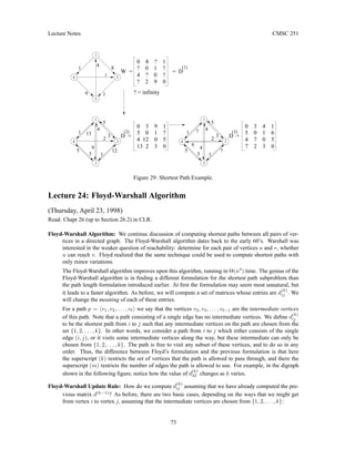
![Lecture Notes CMSC 251
3,2
d = INF
(0)
3,2
d = 12
(1)
3,2
d = 12
(2)
3,2
d = 12
(3)
3,2
(4)
8
d = 7
Vertices 1 through k−1
kj
d
(k−1)
ik
d
(k−1)
k
(a)
(3,1,4,2)
(3,1,2)
(3,1,2)
(3,1,2)
(no path)
9
ij
d
(k−1)
j
i
2 2
1
4
1
4
3
1
Figure 30: Floyd-Warshall Formulation.
We don’t go through k at all: Then the shortest path from i to j uses only intermediate vertices
{1, . . . , k − 1} and hence the length of the shortest path is d
(k−1)
ij .
We do go through k: First observe that a shortest path does not pass through the same vertex twice, so
we can assume that we pass through k exactly once. (The assumption that there are no negative
cost cycles is being used here.) That is, we go from i to k, and then from k to j. In order
for the overall path to be as short as possible we should take the shortest path from i to k, and
the shortest path from k to j. (This is the principle of optimality.) Each of these paths uses
intermediate vertices only in {1, 2, . . . , k − 1}. The length of the path is d
(k−1)
ik + d
(k−1)
kj .
This suggests the following recursive rule for computing d(k)
:
d
(0)
ij = wij,
d
(k)
ij = min
d
(k−1)
ij , d
(k−1)
ik + d
(k−1)
kj
for k ≥ 1.
The final answer is d
(n)
ij because this allows all possible vertices as intermediate vertices. Again, we
could write a recursive program to compute d
(k)
ij , but this will be prohibitively slow. Instead, we
compute it by storing the values in a table, and looking the values up as we need them. Here is the
complete algorithm. We have also included predecessor pointers, pred[i, j] for extracting the final
shortest paths. We will discuss them later.
Floyd-Warshall Algorithm
Floyd_Warshall(int n, int W[1..n, 1..n]) {
array d[1..n, 1..n]
for i = 1 to n do { // initialize
for j = 1 to n do {
d[i,j] = W[i,j]
pred[i,j] = null
}
}
for k = 1 to n do // use intermediates {1..k}
for i = 1 to n do // ...from i
for j = 1 to n do // ...to j
if (d[i,k] + d[k,j]) d[i,j]) {
d[i,j] = d[i,k] + d[k,j] // new shorter path length
pred[i,j] = k // new path is through k
74](https://image.slidesharecdn.com/251-alogarithmslects-230702222135-b89653fc/85/251-Alogarithms-Lects-pdf-74-320.jpg)
![Lecture Notes CMSC 251
}
return d // matrix of final distances
}
Clearly the algorithm’s running time is Θ(n3
). The space used by the algorithm is Θ(n2
). Observe
that we deleted all references to the superscript (k) in the code. It is left as an exercise that this does
not affect the correctness of the algorithm. An example is shown in the following figure.
2
1
3
4
4
3
D =
D =
(3)
(1)
1
2
3
4
4
5
D =
(4)
1 8
1
2
3
4
1
2
3
4
D =
(2)
(0)
1
2
1
5
3
7
3
2
7
3
6
5
8
2
12
9
5
6
7
12
9
5
1
D =
9
4 4
2
8
1
2
4
8
1
4
1
1
3
4
5
1
2
1
9
12
1
5 0 1 6
4 7 0 5
7 2 3 0
0 8 9 1
? 0 1 ?
4 12 0 5
? 2 3 0
0 3 4 1
? = infinity
0 8 ? 1
? 0 1 ?
4 ? 0 ?
? 2 9 0
0 8 ? 1
? 0 1 ?
4 12 0 5
? 2 9 0
0 8 9 1
5 0 1 6
4 12 0 5
7 2 3 0
Figure 31: Floyd-Warshall Example.
Extracting Shortest Paths: The predecessor pointers pred[i, j] can be used to extract the final path. Here
is the idea, whenever we discover that the shortest path from i to j passes through an intermediate
vertex k, we set pred[i, j] = k. If the shortest path does not pass through any intermediate vertex,
then pred[i, j] = null. To find the shortest path from i to j, we consult pred[i, j]. If it is null, then
the shortest path is just the edge (i, j). Otherwise, we recursively compute the shortest path from i to
pred[i, j] and the shortest path from pred[i, j] to j.
Printing the Shortest Path
Path(i,j) {
if pred[i,j] = null // path is a single edge
output(i,j)
else { // path goes through pred
Path(i, pred[i,j]); // print path from i to pred
Path(pred[i,j], j); // print path from pred to j
}
}
75](https://image.slidesharecdn.com/251-alogarithmslects-230702222135-b89653fc/85/251-Alogarithms-Lects-pdf-75-320.jpg)
![Lecture Notes CMSC 251
Lecture 25: Longest Common Subsequence
(April 28, 1998)
Read: Section 16.3 in CLR.
Strings: One important area of algorithm design is the study of algorithms for character strings. There are
a number of important problems here. Among the most important has to do with efficiently searching
for a substring or generally a pattern in large piece of text. (This is what text editors and functions
like ”grep” do when you perform a search.) In many instances you do not want to find a piece of text
exactly, but rather something that is ”similar”. This arises for example in genetics research. Genetic
codes are stored as long DNA molecules. The DNA strands can be broken down into a long sequences
each of which is one of four basic types: C, G, T, A.
But exact matches rarely occur in biology because of small changes in DNA replication. Exact sub-
string search will only find exact matches. For this reason, it is of interest to compute similarities
between strings that do not match exactly. The method of string similarities should be insensitive to
random insertions and deletions of characters from some originating string. There are a number of
measures of similarity in strings. The first is the edit distance, that is, the minimum number of single
character insertions, deletions, or transpositions necessary to convert one string into another. The other,
which we will study today, is that of determining the length of the longest common subsequence.
Longest Common Subsequence: Let us think of character strings as sequences of characters. Given two
sequences X = hx1, x2, . . . , xmi and Z = hz1, z2, . . . , zki, we say that Z is a subsequence of X if
there is a strictly increasing sequence of k indices hi1, i2, . . . , iki (1 ≤ i1 i2 . . . ik ≤ n) such
that Z = hXi1
, Xi2
, . . . , Xik
i. For example, let X = hABRACADABRAi and let Z = hAADAAi,
then Z is a subsequence of X.
Given two strings X and Y , the longest common subsequence of X and Y is a longest sequence Z
which is both a subsequence of X and Y .
For example, let X be as before and let Y = hYABBADABBADOOi. Then the longest common
subsequence is Z = hABADABAi.
The Longest Common Subsequence Problem (LCS) is the following. Given two sequences X =
hx1, . . . , xmi and Y = hy1, . . . , yni determine a longest common subsequence. Note that it is not
always unique. For example the LCS of hABCi and hBACi is either hACi or hBCi.
Dynamic Programming Solution: The simple brute-force solution to the problem would be to try all pos-
sible subsequences from one string, and search for matches in the other string, but this is hopelessly
inefficient, since there are an exponential number of possible subsequences.
Instead, we will derive a dynamic programming solution. In typical DP fashion, we need to break the
problem into smaller pieces. There are many ways to do this for strings, but it turns out for this problem
that considering all pairs of prefixes will suffice for us. A prefix of a sequence is just an initial string of
values, Xi = hx1, x2, . . . , xii. X0 is the empty sequence.
The idea will be to compute the longest common subsequence for every possible pair of prefixes. Let
c[i, j] denote the length of the longest common subsequence of Xi and Yj. Eventually we are interested
in c[m, n] since this will be the LCS of the two entire strings. The idea is to compute c[i, j] assuming
that we already know the values of c[i0
, j0
] for i0
≤ i and j0
≤ j (but not both equal). We begin with
some observations.
Basis: c[i, 0] = c[j, 0] = 0. If either sequence is empty, then the longest common subsequence is
empty.
76](https://image.slidesharecdn.com/251-alogarithmslects-230702222135-b89653fc/85/251-Alogarithms-Lects-pdf-76-320.jpg)
![Lecture Notes CMSC 251
Last characters match: Suppose xi = yj. Example: Let Xi = hABCAi and let Yj = hDACAi.
Since both end in A, we claim that the LCS must also end in A. (We will explain why later.)
Since the A is part of the LCS we may find the overall LCS by removing A from both sequences
and taking the LCS of Xi−1 = hABCi and Yj−1 = hDACi which is hACi and then adding A
to the end, giving hACAi as the answer. (At first you might object: But how did you know that
these two A’s matched with each other. The answer is that we don’t, but it will not make the LCS
any smaller if we do.)
Thus, if xi = yj then c[i, j] = c[i − 1, j − 1] + 1.
Last characters do not match: Suppose that xi 6= yj. In this case xi and yj cannot both be in the
LCS (since they would have to be the last character of the LCS). Thus either xi is not part of the
LCS, or yj is not part of the LCS (and possibly both are not part of the LCS).
In the first case the LCS of Xi and Yj is the LCS of Xi−1 and Yj, which is c[i − 1, j]. In the
second case the LCS is the LCS of Xi and Yj−1 which is c[i, j − 1]. We do not know which is
the case, so we try both and take the one that gives us the longer LCS.
Thus, if xi 6= yj then c[i, j] = max(c[i − 1, j], c[i, j − 1]).
We left undone the business of showing that if both strings end in the same character, then the LCS
must also end in this same character. To see this, suppose by contradiction that both characters end in
A, and further suppose that the LCS ended in a different character B. Because A is the last character
of both strings, it follows that this particular instance of the character A cannot be used anywhere else
in the LCS. Thus, we can add it to the end of the LCS, creating a longer common subsequence. But
this would contradict the definition of the LCS as being longest.
Combining these observations we have the following rule:
c[i, j] =
0 if i = 0 or j = 0,
c[i − 1, j − 1] + 1 if i, j 0 and xi = yj,
max(c[i, j − 1], c[i − 1, j]) if i, j 0 and xi 6= yj.
Implementing the Rule: The task now is to simply implement this rule. As with other DP solutions, we
concentrate on computing the maximum length. We will store some helpful pointers in a parallel array,
b[0..m, 0..n].
Longest Common Subsequence
LCS(char x[1..m], char y[1..n]) {
int c[0..m, 0..n]
for i = 0 to m do {
c[i,0] = 0 b[i,0] = SKIPX // initialize column 0
}
for j = 0 to n do {
c[0,j] = 0 b[0,j] = SKIPY // initialize row 0
}
for i = 1 to m do {
for j = 1 to n do {
if (x[i] == y[j]) {
c[i,j] = c[i-1,j-1]+1 // take X[i] and Y[j] for LCS
b[i,j] = ADDXY
}
else if (c[i-1,j] = c[i,j-1]) { // X[i] not in LCS
c[i,j] = c[i-1,j]
b[i,j] = SKIPX
}
else { // Y[j] not in LCS
77](https://image.slidesharecdn.com/251-alogarithmslects-230702222135-b89653fc/85/251-Alogarithms-Lects-pdf-77-320.jpg)
![Lecture Notes CMSC 251
c[i,j] = c[i,j-1]
b[i,j] = SKIPY
}
}
}
return c[m,n];
}
LCS Length Table with back pointers included
m=
=n
3
2
2
1
2
2
1 2
2
1 1
1 2
1
0
0
0
0
B
D
C
B
A
B
C
D
B
4
3
2
1
0
4
3
2
1
5 start here
A
B
C
D
B
4
3
2
1
0
4
3
2
1
0
5
m=
=n
B
1
1
1
1
1
1
0
0
0
0
0
0
0
0
0
0
B
D
C
0
1
2
2
1
1
1
1
1
1
1
1
1
1
0
0
0
0
0
0
2
X = BACDB
Y = BDCB
LCS = BCB
3
2
2
1
2
2
Figure 32: Longest common subsequence example.
The running time of the algorithm is clearly O(mn) since there are two nested loops with m and n
iterations, respectively. The algorithm also uses O(mn) space.
Extracting the Actual Sequence: Extracting the final LCS is done by using the back pointers stored in
b[0..m, 0..n]. Intuitively b[i, j] = ADDXY means that X[i] and Y [j] together form the last character
of the LCS. So we take this common character, and continue with entry b[i − 1, j − 1] to the northwest
(-). If b[i, j] = SKIPX , then we know that X[i] is not in the LCS, and so we skip it and go to
b[i − 1, j] above us (↑). Similarly, if b[i, j] = SKIPY , then we know that Y [j] is not in the LCS,
and so we skip it and go to b[i, j − 1] to the left (←). Following these back pointers, and outputting a
character with each diagonal move gives the final subsequence.
Print Subsequence
getLCS(char x[1..m], char y[1..n], int b[0..m,0..n]) {
LCS = empty string
i = m
j = n
while(i != 0 j != 0) {
switch b[i,j] {
case ADDXY:
add x[i] (or equivalently y[j]) to front of LCS
i--; j--; break
case SKIPX:
i--; break
case SKIPY:
j--; break
}
}
return LCS
}
78](https://image.slidesharecdn.com/251-alogarithmslects-230702222135-b89653fc/85/251-Alogarithms-Lects-pdf-78-320.jpg)
![Lecture Notes CMSC 251
Lecture 26: Chain Matrix Multiplication
(Thursday, April 30, 1998)
Read: Section 16.1 of CLR.
Chain Matrix Multiplication: This problem involves the question of determining the optimal sequence for
performing a series of operations. This general class of problem is important in compiler design for
code optimization and in databases for query optimization. We will study the problem in a very re-
stricted instance, where the dynamic programming issues are easiest to see.
Suppose that we wish to multiply a series of matrices
A1A2 . . . An
Matrix multiplication is an associative but not a commutative operation. This means that we are free to
parenthesize the above multiplication however we like, but we are not free to rearrange the order of the
matrices. Also recall that when two (nonsquare) matrices are being multiplied, there are restrictions on
the dimensions. A p × q matrix has p rows and q columns. You can multiply a p × q matrix A times a
q × r matrix B, and the result will be a p × r matrix C. (The number of columns of A must equal the
number of rows of B.) In particular for 1 ≤ i ≤ p and 1 ≤ j ≤ r,
C[i, j] =
q
X
k=1
A[i, k]B[k, j].
Observe that there are pr total entries in C and each takes O(q) time to compute, thus the total time
(e.g. number of multiplications) to multiply these two matrices is p · q · r.
B C
=
A
p
q
q
r
p
r
Multiplication
pqr
time =
=
*
Figure 33: Matrix Multiplication.
Note that although any legal parenthesization will lead to a valid result, not all involve the same number
of operations. Consider the case of 3 matrices: A1 be 5 × 4, A2 be 4 × 6 and A3 be 6 × 2.
mult[((A1A2)A3)] = (5 · 4 · 6) + (5 · 6 · 2) = 180,
mult[(A1(A2A3))] = (4 · 6 · 2) + (5 · 4 · 2) = 88.
Even for this small example, considerable savings can be achieved by reordering the evaluation se-
quence. The Chain Matrix Multiplication problem is: Given a sequence of matrices A1, A2, . . . , An
and dimensions p0, p1, . . . , pn where Ai is of dimension pi−1 × pi, determine the multiplication se-
quence that minimizes the number of operations.
Important Note: This algorithm does not perform the multiplications, it just figures out the best order
in which to perform the multiplications.
79](https://image.slidesharecdn.com/251-alogarithmslects-230702222135-b89653fc/85/251-Alogarithms-Lects-pdf-79-320.jpg)
![Lecture Notes CMSC 251
Naive Algorithm: We could write a procedure which tries all possible parenthesizations. Unfortunately, the
number of ways of parenthesizing an expression is very large. If you have just one item, then there is
only one way to parenthesize. If you have n items, then there are n − 1 places where you could break
the list with the outermost pair of parentheses, namely just after the 1st item, just after the 2nd item,
etc., and just after the (n − 1)st item. When we split just after the kth item, we create two sublists to
be parenthesized, one with k items, and the other with n − k items. Then we could consider all the
ways of parenthesizing these. Since these are independent choices, if there are L ways to parenthesize
the left sublist and R ways to parenthesize the right sublist, then the total is L · R. This suggests the
following recurrence for P(n), the number of different ways of parenthesizing n items:
P(n) =
1 if n = 1,
Pn−1
k=1 P(k)P(n − k) if n ≥ 2.
This is related to a famous function in combinatorics called the Catalan numbers (which in turn is
related to the number of different binary trees on n nodes). In particular P(n) = C(n − 1) and
C(n) =
1
n + 1
2n
n
.
Applying Stirling’s formula, we find that C(n) ∈ Ω(4n
/n3/2
). Since 4n
is exponential and n3/2
is just
polynomial, the exponential will dominate, and this grows very fast. Thus, this will not be practical
except for very small n.
Dynamic Programming Solution: This problem, like other dynamic programming problems involves de-
termining a structure (in this case, a parenthesization). We want to break the problem into subproblems,
whose solutions can be combined to solve the global problem.
For convenience we can write Ai..j to be the product of matrices i through j. It is easy to see that
Ai..j is a pi−1 × pj matrix. In parenthesizing the expression, we can consider the highest level of
parenthesization. At this level we are simply multiplying two matrices together. That is, for any k,
1 ≤ k ≤ n − 1,
A1..n = A1..kAk+1..n.
Thus the problem of determining the optimal sequence of multiplications is broken up into 2 questions:
how do we decide where to split the chain (what is k?) and how do we parenthesize the subchains
A1..k and Ak+1..n? The subchain problems can be solved by recursively applying the same scheme.
The former problem can be solved by just considering all possible values of k. Notice that this problem
satisfies the principle of optimality, because if we want to find the optimal sequence for multiplying
A1..n we must use the optimal sequences for A1..k and Ak+1..n. In other words, the subproblems must
be solved optimally for the global problem to be solved optimally.
We will store the solutions to the subproblems in a table, and build the table in a bottom-up manner.
For 1 ≤ i ≤ j ≤ n, let m[i, j] denote the minimum number of multiplications needed to compute
Ai..j. The optimum cost can be described by the following recursive definition. As a basis observe that
if i = j then the sequence contains only one matrix, and so the cost is 0. (There is nothing to multiply.)
Thus, m[i, i] = 0. If i j, then we are asking about the product Ai..j. This can be split by considering
each k, i ≤ k j, as Ai..k times Ak+1..j.
The optimum time to compute Ai..k is m[i, k], and the optimum time to compute Ak+1..j is m[k+1, j].
We may assume that these values have been computed previously and stored in our array. Since Ai..k
is a pi−1 × pk matrix, and Ak+1..j is a pk × pj matrix, the time to multiply them is pi−1 · pk · pj. This
suggests the following recursive rule for computing m[i, j].
m[i, i] = 0
m[i, j] = min
i≤kj
(m[i, k] + m[k + 1, j] + pi−1pkpj) for i j.
80](https://image.slidesharecdn.com/251-alogarithmslects-230702222135-b89653fc/85/251-Alogarithms-Lects-pdf-80-320.jpg)
![Lecture Notes CMSC 251
It is not hard to convert this rule into a procedure, which is given below. The only tricky part is arranging
the order in which to compute the values. In the process of computing m[i, j] we will need to access
values m[i, k] and m[k+1, j] for k lying between i and j. This suggests that we should organize things
our computation according to the number of matrices in the subchain. Let L = j − i + 1 denote the
length of the subchain being multiplied. The subchains of length 1 (m[i, i]) are trivial. Then we build
up by computing the subchains of lengths 2, 3, . . . , n. The final answer is m[1, n]. We need to be a
little careful in setting up the loops. If a subchain of length L starts at position i, then j = i + L − 1.
Since we want j ≤ n, this means that i + L − 1 ≤ n, or in other words, i ≤ n − L + 1. So our loop
for i runs from 1 to n − L + 1 (to keep j in bounds).
Chain Matrix Multiplication
Matrix-Chain(array p[1..n], int n) {
array s[1..n-1,2..n]
for i = 1 to n do m[i,i] = 0 // initialize
for L = 2 to n do { // L = length of subchain
for i = 1 to n-L+1 do {
j = i + L - 1
m[i,j] = INFINITY
for k = i to j-1 do {
q = m[i, k] + m[k+1, j] + p[i-1]*p[k]*p[j]
if (q m[i, j]) { m[i,j] = q; s[i,j] = k }
}
}
}
return m[1,n] and s
}
The array s[i, j] will be explained later. It is used to extract the actual sequence. The running time of
the procedure is Θ(n3
). We’ll leave this as an exercise in solving sums, but the key is that there are
three nested loops, and each can iterate at most n times.
Extracting the final Sequence: To extract the actual sequence is a fairly easy extension. The basic idea is
to leave a split marker indicating what the best split is, that is, what value of k lead to the minimum
value of m[i, j]. We can maintain a parallel array s[i, j] in which we will store the value of k providing
the optimal split. For example, suppose that s[i, j] = k. This tells us that the best way to multiply
the subchain Ai..j is to first multiply the subchain Ai..k and then multiply the subchain Ak+1..j, and
finally multiply these together. Intuitively, s[i, j] tells us what multiplication to perform last. Note that
we only need to store s[i, j] when we have at least two matrices, that is, if j i.
The actual multiplication algorithm uses the s[i, j] value to determine how to split the current sequence.
Assume that the matrices are stored in an array of matrices A[1..n], and that s[i, j] is global to this
recursive procedure. The procedure returns a matrix.
Extracting Optimum Sequence
Mult(i, j) {
if (i j) {
k = s[i,j]
X = Mult(i, k) // X = A[i]...A[k]
Y = Mult(k+1, j) // Y = A[k+1]...A[j]
return X*Y; // multiply matrices X and Y
}
else
return A[i];
}
81](https://image.slidesharecdn.com/251-alogarithmslects-230702222135-b89653fc/85/251-Alogarithms-Lects-pdf-81-320.jpg)
![Lecture Notes CMSC 251
i
0
j
7
2
6
4
1
2
3
4 1
2
3
4
0
p 4
p
3
p
2
p
1
p
m[i,j]
5
158
88
120 48
104
84
0
0
0
Final order
3
4
A
3
A
2
A
1
A
4
A
3
A
2
A
1
A
2
3
2
1
1
3
3
1
3
2
1
s[i,j]
i
j
2
3
4
Figure 34: Chain Matrix Multiplication.
In the figure below we show an example. This algorithm is tricky, so it would be a good idea to trace
through this example (and the one given in the text). The initial set of dimensions are h5, 4, 6, 2, 7i
meaning that we are multiplying A1 (5 × 4) times A2 (4 × 6) times A3 (6 × 2) times A4 (2 × 7). The
optimal sequence is ((A1(A2A3))A4).
Lecture 27: NP-Completeness: General Introduction
(Tuesday, May 5, 1998)
Read: Chapt 36, up through section 36.4.
Easy and Hard Problems: At this point of the semester hopefully you have learned a few things of what
it means for an algorithm to be efficient, and how to design algorithms and determine their efficiency
asymptotically. All of this is fine if it helps you discover an acceptably efficient algorithm to solve
your problem. The question that often arises in practice is that you have tried every trick in the book,
and still your best algorithm is not fast enough. Although your algorithm can solve small problems
reasonably efficiently (e.g. n ≤ 20) the really large applications that you want to solve (e.g. n ≥ 100)
your algorithm does not terminate quickly enough. When you analyze its running time, you realize that
it is running in exponential time, perhaps n
√
n
, or 2n
, or 2(2n
)
, or n!, or worse.
Towards the end of the 60’s and in the eary 70’s there were great strides made in finding efficient
solutions to many combinatorial problems. But at the same time there was also a growing list of
problems for which there seemed to be no known efficient algorithmic solutions. The best solutions
known for these problems required exponential time. People began to wonder whether there was some
unknown paradigm that would lead to a solution to these problems, or perhaps some proof that these
problems are inherently hard to solve and no algorithmic solutions exist that run under exponential
time.
Around this time a remarkable discovery was made. It turns out that many of these “hard” problems
were interrelated in the sense that if you could solve any one of them in polynomial time, then you
could solve all of them in polynomial time. The next couple of lectures we will discuss some of these
problems and introduce the notion of P, NP, and NP-completeness.
Polynomial Time: We need some way to separate the class of efficiently solvable problems from ineffi-
ciently solvable problems. We will do this by considering problems that can be solved in polynomial
time.
82](https://image.slidesharecdn.com/251-alogarithmslects-230702222135-b89653fc/85/251-Alogarithms-Lects-pdf-82-320.jpg)
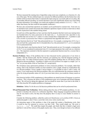
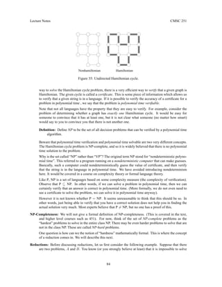
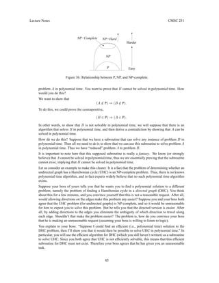
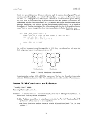
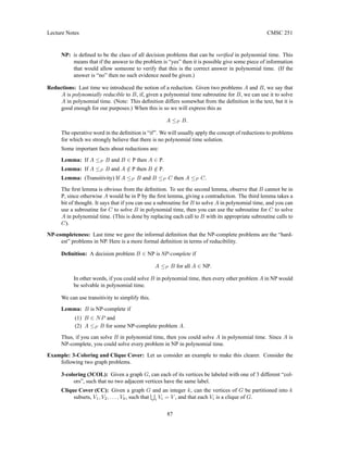
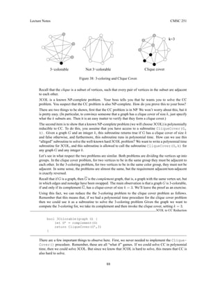
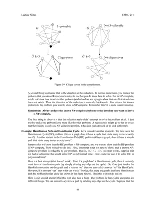
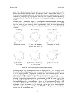
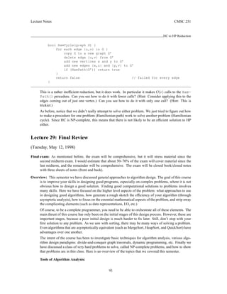
![Lecture Notes CMSC 251
Asymptotics: O, Ω, Θ. General facts about growth rates of functions.
Summations: Analysis of looping programs, common summations, solving complex summa-
tions, integral approximation, constructive induction.
Recurrences: Analysis of recursive programs, strong induction, expansion, Master Theorem.
Sorting:
Mergesort: Stable, Θ(n log n) sorting algorithm.
Heapsort: Nonstable, Θ(n log n), in-place algorithm. A heap is an important data structure for
implementation of priority queues (a queue in which the highest priority item is dequeued
first).
Quicksort: Nonstable, Θ(n log n) expected case, (almost) in-place sorting algorithm. This is
regarded as the fastest of these sorting algorithms, primarily because of its pattern of locality
of reference.
Sorting lower bounds: Any sorting algorithm that is based on comparisons requires Ω(n log n)
steps in the worst-case. The argument is based on a decision tree. Considering the number
of possible outcomes, and observe that they form the leaves of the decision tree. The height
of the decision tree is Ω(lg N), where N is the number of leaves. In this case, N = n!, the
number of different permutations of n keys.
Linear time sorting: If you are sorting small integers in the range from 1 to k, then you can
applying counting sort in Θ(n + k) time. If k is too large, then you can try breaking the
numbers up into smaller digits, and apply radix sort instead. Radix sort just applies counting
sort to each digit individually. If there are d digits, then its running time is Θ(d(n + k)),
where k is the number of different values in each digit.
Graphs: We presented basic definitions of graphs and digraphs. A graph (digraph) consists of a set
of vertices and a set of undirected (directed) edges. Recall that the number of edges in a graph
can generally be as large as O(n2
), but is often smaller (closer to O(n)). A graph is sparse if the
number of edges is o(n2
), and dense otherwise.
We discussed two representations:
Adjacency matrix: A[u, v] = 1 if (u, v) ∈ E. These are simple, but require Θ(n2
) storage.
Good for dense graphs.
Adjacency list: Adj[u] is a pointer to a linked list containing the neighbors of u. These are better
for sparse graphs, since they only require Θ(n + e) storage.
Breadth-first search: We discussed one graph algorithm: breadth first search. This is a way of
traversing the vertices of a graph in increasing order of distance from a source vertex. Recall
that it colors vertices (white, gray, black) to indicate their status in the search, and it also uses a
FIFO queue to determine which order it will visit the vertices. When we process the next vertex,
we simply visit (that is, enqueue) all of its unvisited neighbors. This runs in Θ(n + e) time. (If
the queue is replaced by a stack, then we get a different type of search algorithm, called depth-
first search.) We showed that breadth-first search could be used to compute shortest paths from a
single source vertex in an (unweighted) graph or digraph.
Dynamic Programming: Dynamic programming is an important design technique used in many op-
timization problems. Its basic elements are those of subdividing large complex problems into
smaller subproblems, solving subproblems in a bottom-up manner (going from smaller to larger).
An important idea in dynamic programming is that of the principal of optimality: For the global
problem to be solved optimally, the subproblems should be solved optimally. This is not always
the case (e.g., when there is dependence between the subproblems, it might be better to do worse
and one to get a big savings on the other).
Floyd-Warshall Algorithm: (Section 26.2) Shortest paths in a weighted digraph between all
pairs of vertices. This algorithm allows negative cost edges, provided that there are no neg-
ative cost cycles. We gave two algorithms. The first was based on a DP formulation of
92](https://image.slidesharecdn.com/251-alogarithmslects-230702222135-b89653fc/85/251-Alogarithms-Lects-pdf-92-320.jpg)
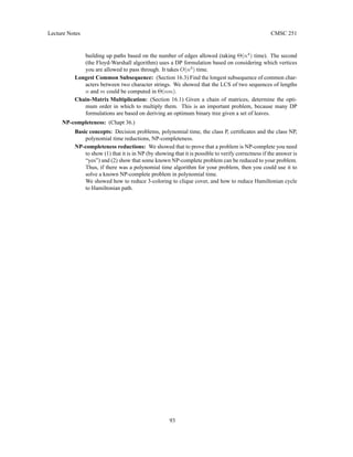

The document summarizes a lecture on algorithms and algorithm design from a course on algorithms. It introduces the concept of algorithms and what will be covered in the course, which includes analyzing algorithms, sorting techniques as a case study, and various algorithmic problems and solutions. It also discusses implementation issues and keeping mathematical analysis independent of specific programming languages or machines. As an example, it analyzes the brute force algorithm for solving the 2D maxima problem in pseudo-code and calculates its running time.