
![19 March 2020 Dr. Abdulfatah Salem 30
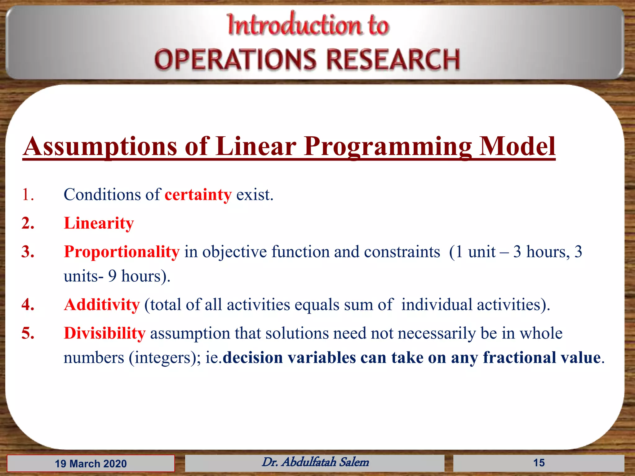
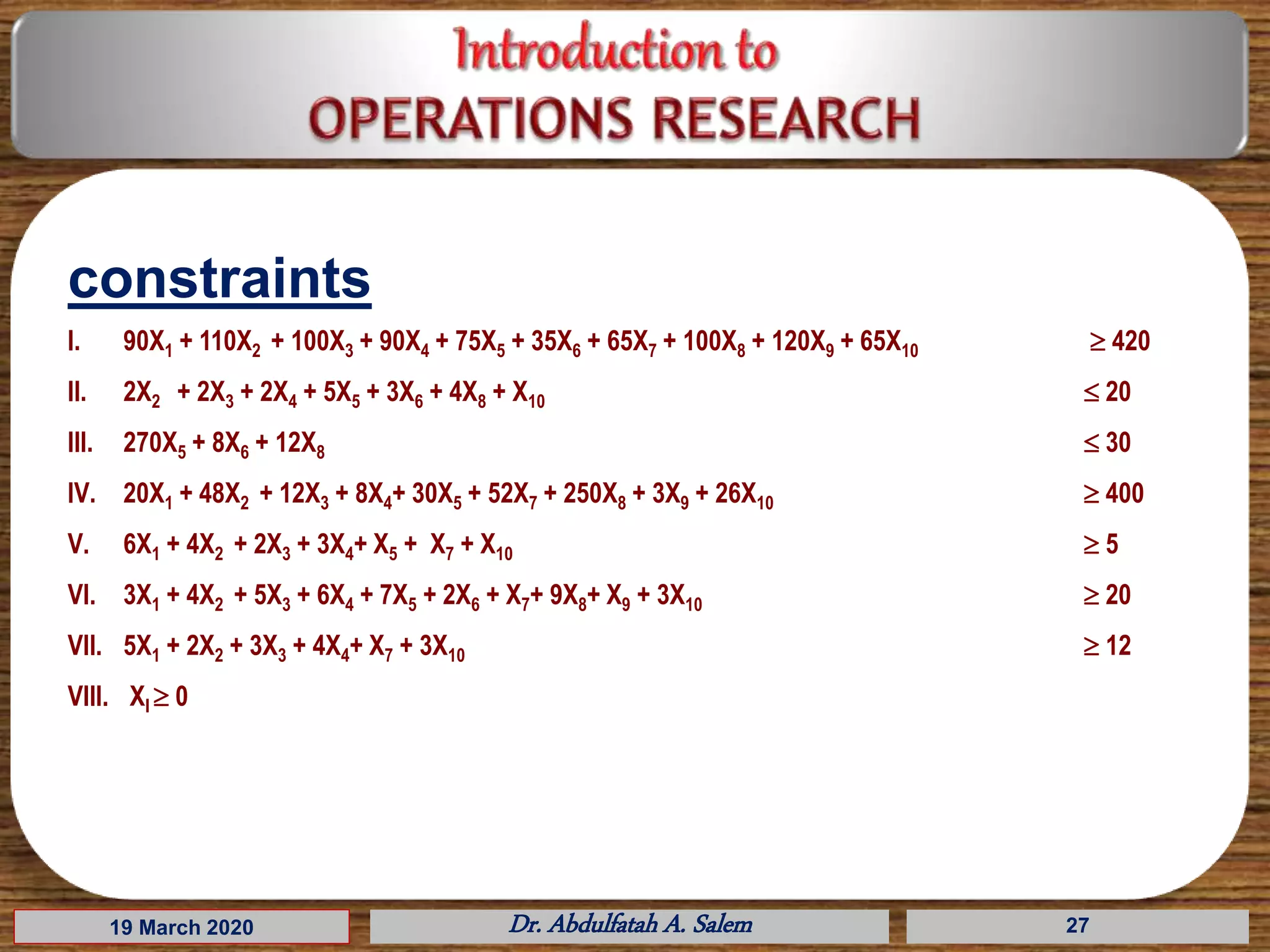
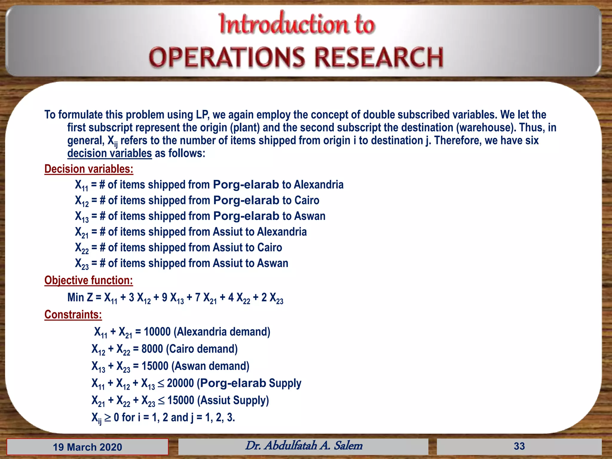
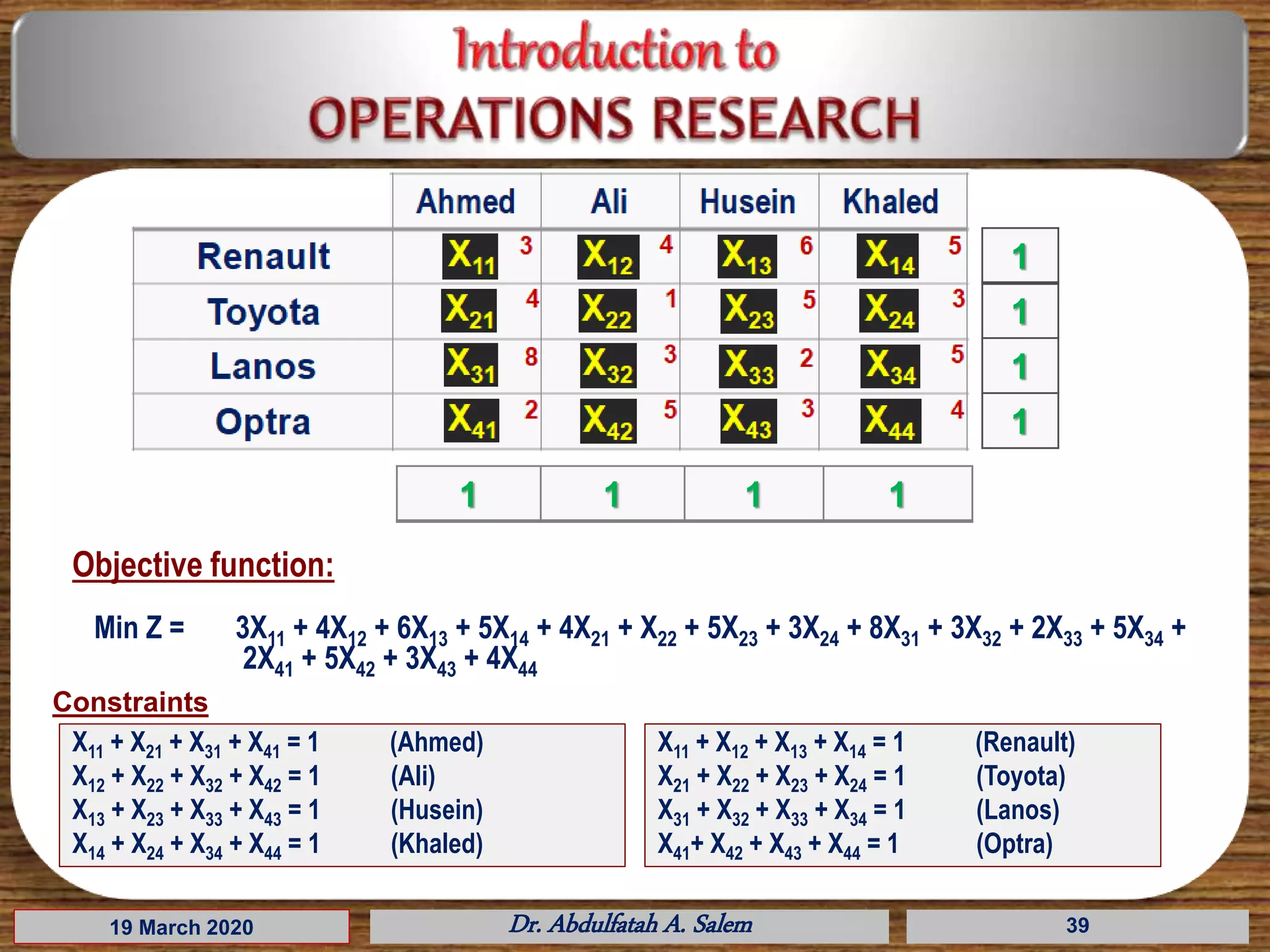
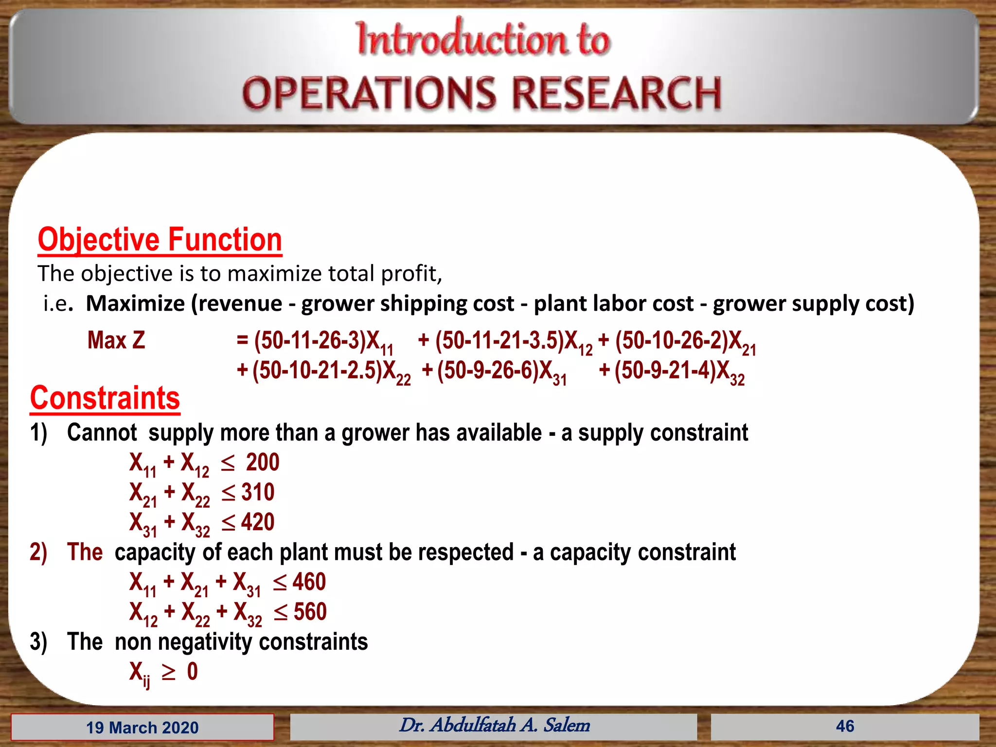
Objective Function
The objective is to maximize total profit Z,
i.e.
Max Z = 310[X11+ X12+X13]
+ 380[X21+ X22+X23]
+ 350[X31+ X32+X33]
+ 285[X41+ X42+X43]](https://image.slidesharecdn.com/introductiontooperationsresearch-200319205849/75/Introduction-to-operations-research-30-2048.jpg)


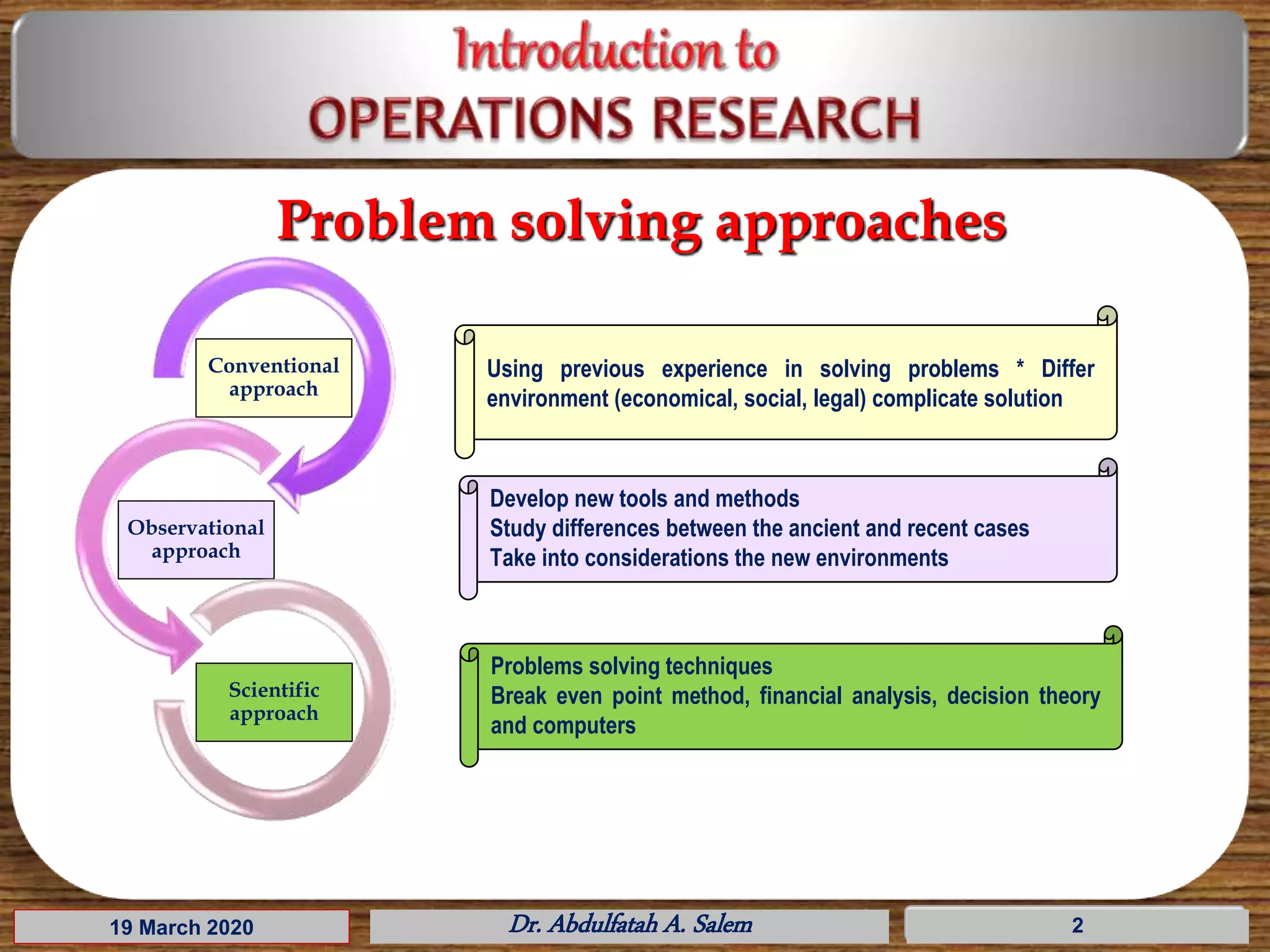
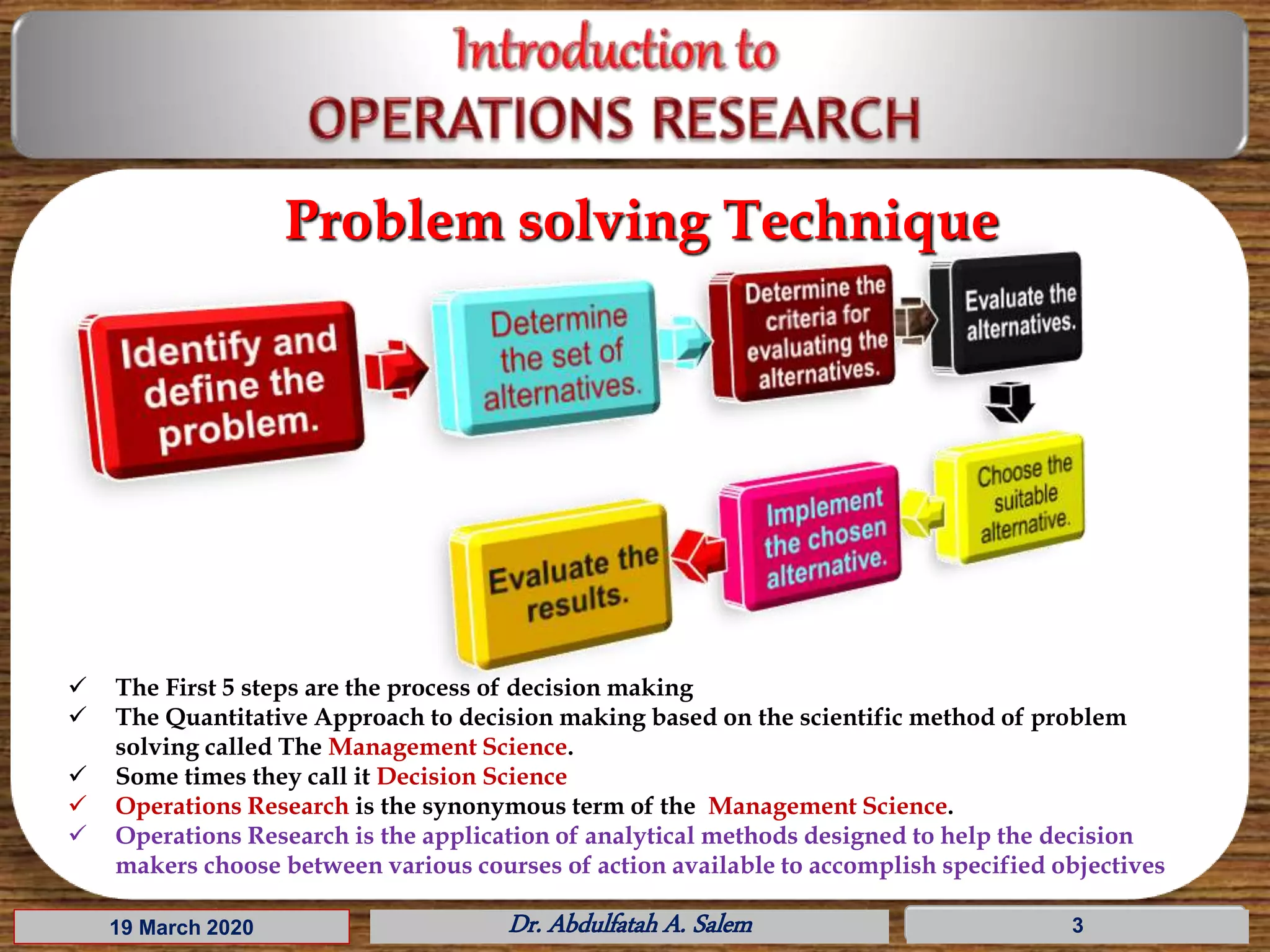
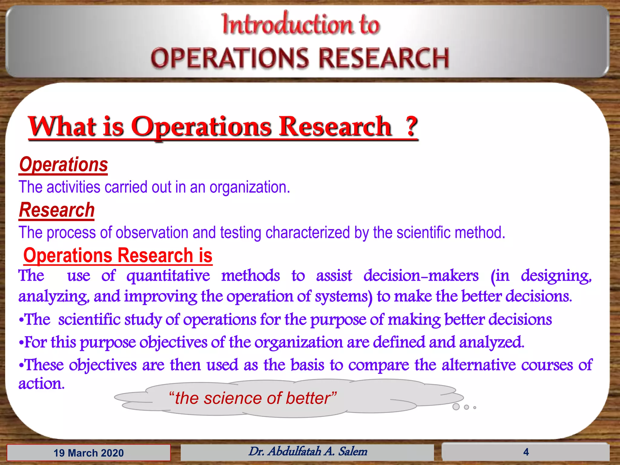
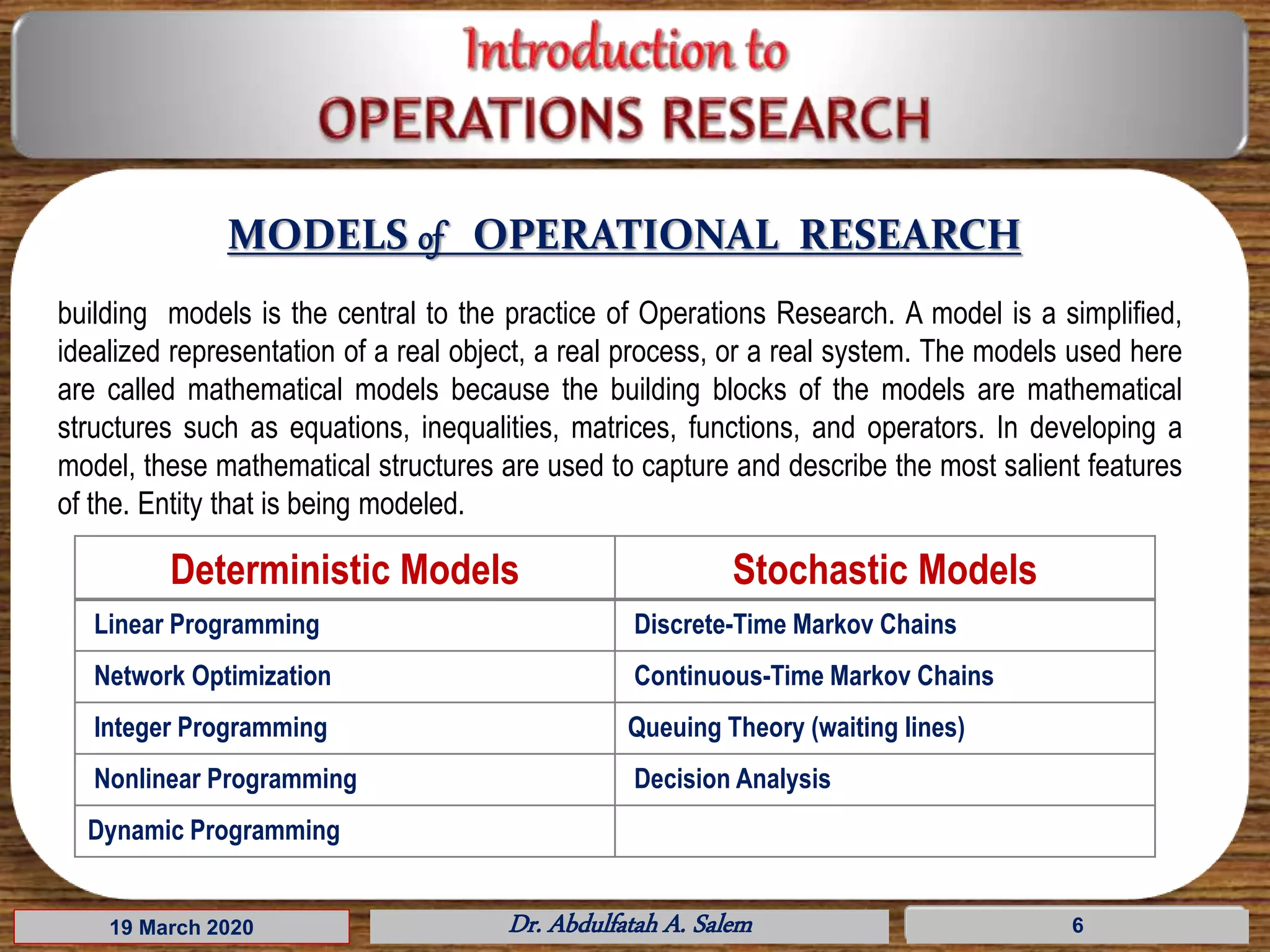
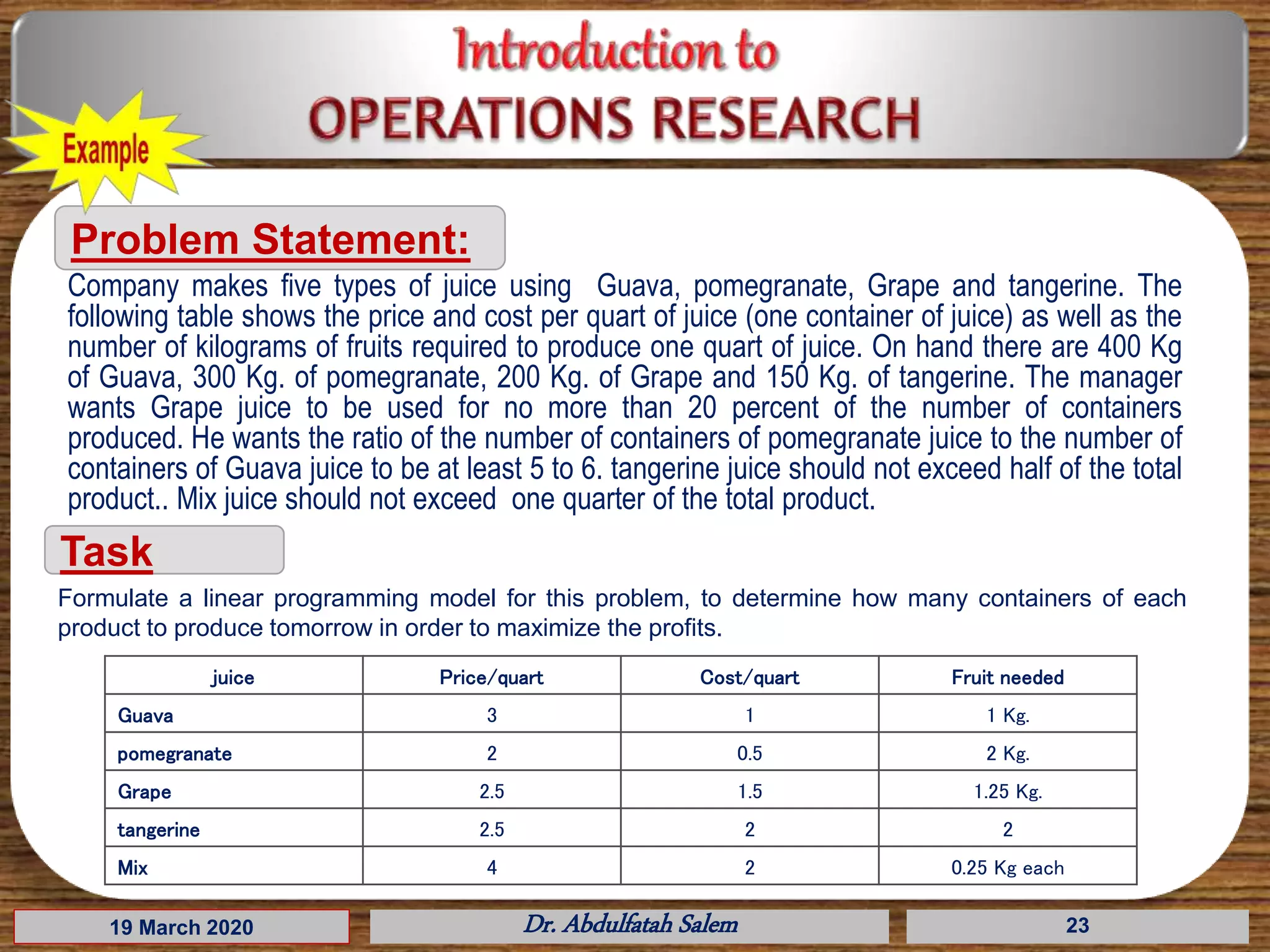
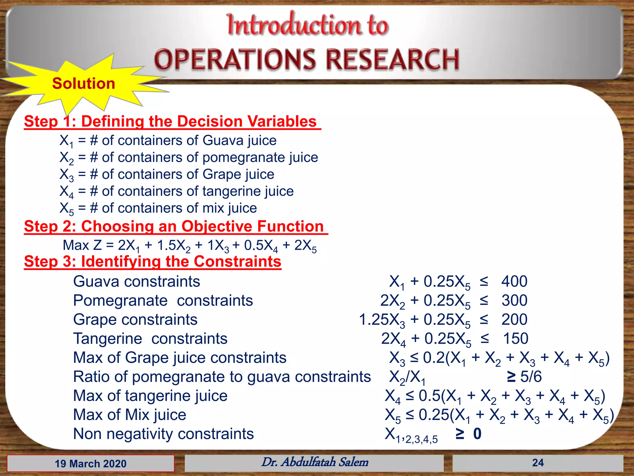
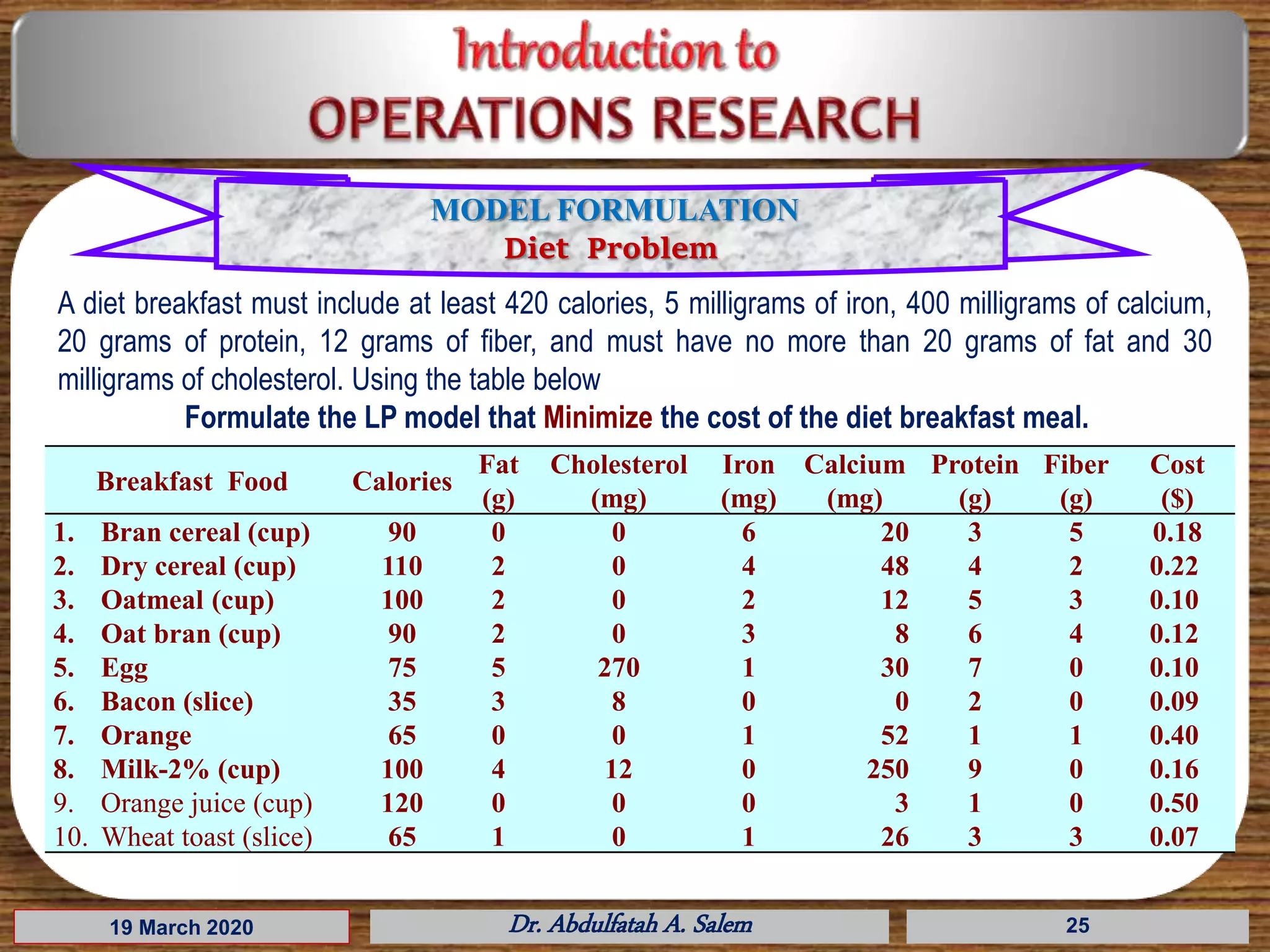
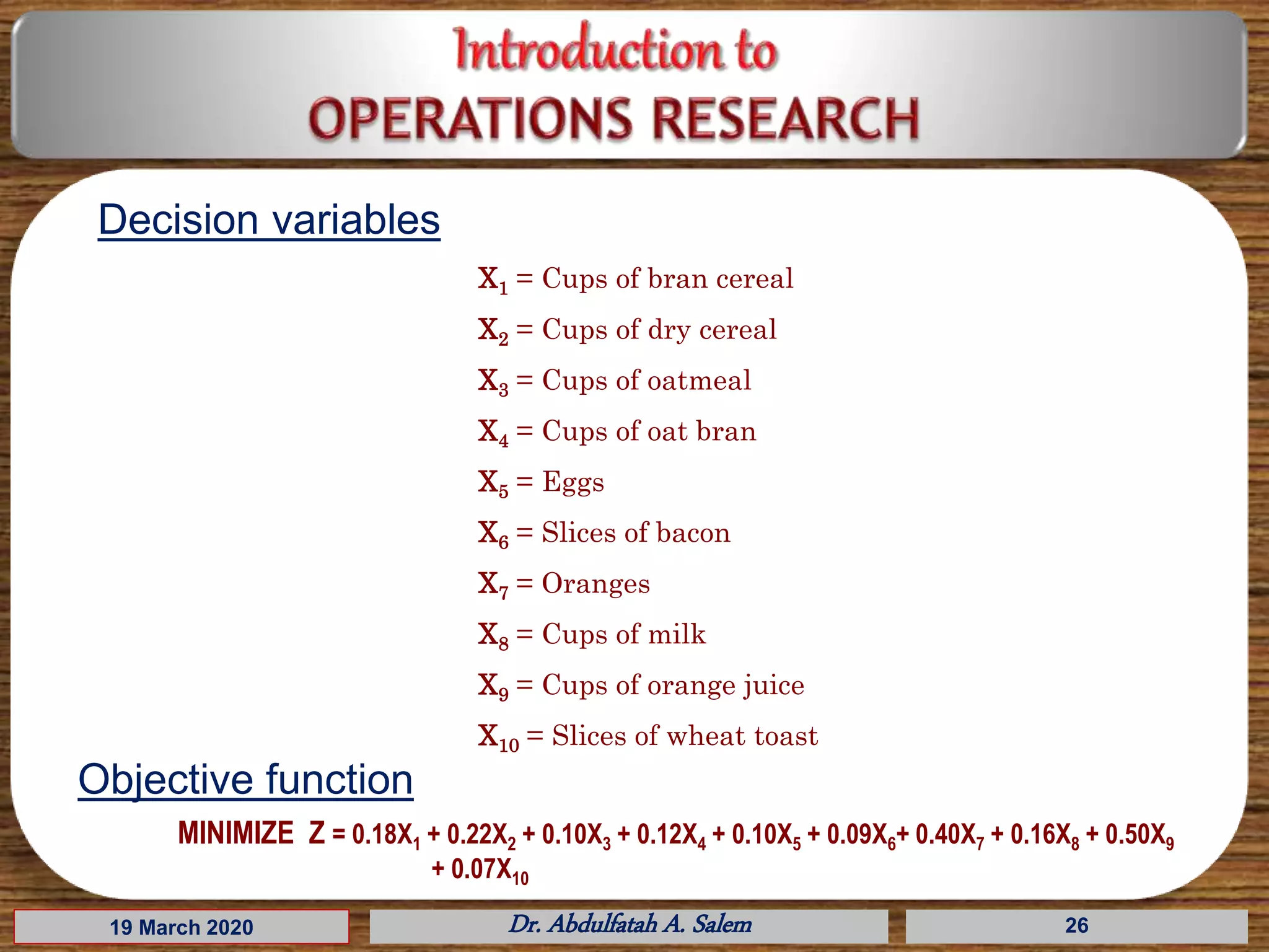
The document discusses problem solving approaches and techniques in operations research. It defines operations research as using quantitative methods to assist decision-makers in designing, analyzing, and improving systems to make better decisions. The scientific approach involves studying differences between past and present cases while considering new environmental factors. Some quantitative techniques mentioned include break-even point analysis, financial analysis, and decision theory. The document also provides examples of linear programming models and their components.