CH-2 Linear Programing.pptx

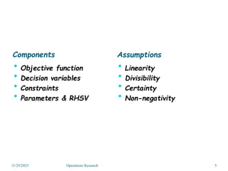
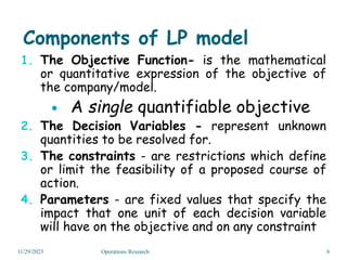
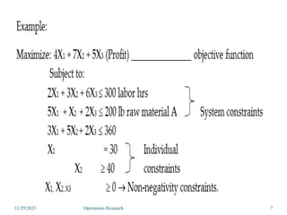
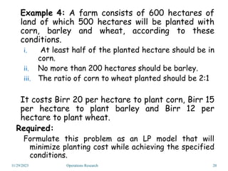
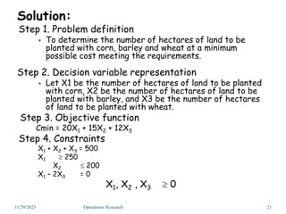
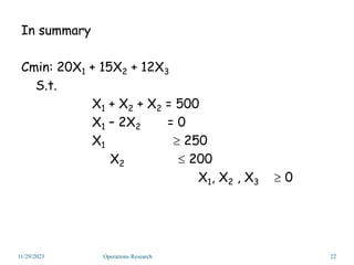
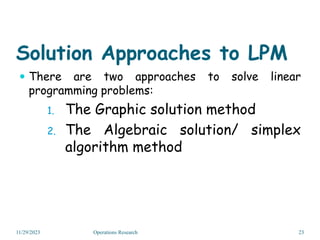
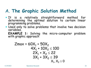
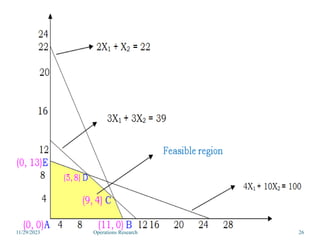
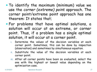
CHAPTER TWO
LINEAR PROGRAMMING
11/29/2023 Operations Research 1

Linear Programming
 Is an optimization method, which shows how to
allocate scarce resources such as money,
materials or time and how to do such allocation in
the best possible way subject to more than one
limiting condition expressed in the form of
inequalities and/or equations.
 It enables to find optimal solution to certain
problems in which the solution must satisfy a
given set of requirements or constraints.
11/29/2023 2
Operations Research

 Optimization in linear programming implies either
 Maximization objective
 Profit, Revenue, Sales, and market share
 Minimization objective
 Cost, time, and distance
 It implies that in LP we cannot max/min two
quantities in one model. It involves linearly related
multi-variate functions, i.e., functions with more
than one independent variable.
 The goal in linear programming is to find the best
solution given the constraints imposed by the
problem; hence the term constrained optimization.
11/29/2023 3
Operations Research

Linear programming Models (LPM)
 Linear Programming (LP) models are mathematical
representations of LP problems.
 The characteristics can be grouped into two
categories: Components and Assumptions.
 The components relate to the structure of a
model, whereas the assumptions reveal the
conditions under which the model is valid.
11/29/2023 4
Operations Research

Components
 Objective function
 Decision variables
 Constraints
 Parameters & RHSV
Assumptions
 Linearity
 Divisibility
 Certainty
 Non-negativity
11/29/2023 5
Operations Research

Components of LP model
1. The Objective Function- is the mathematical
or quantitative expression of the objective of
the company/model.
 A single quantifiable objective
2. The Decision Variables - represent unknown
quantities to be resolved for.
3. The constraints - are restrictions which define
or limit the feasibility of a proposed course of
action.
4. Parameters - are fixed values that specify the
impact that one unit of each decision variable
will have on the objective and on any constraint
11/29/2023 6
Operations Research

11/29/2023 7
Operations Research

Assumption of LP Models
1. Linearity. Each decision variable has a linear
impact on the objective function and in each
constraint.
2. Divisibility : Non-integer values are acceptable.
3. Certainty. model parameters values are known
and constant
4. Non-negativity: Negative values of variables
are unrealistic and, therefore, will not be
considered in any potential solution
11/29/2023 8
Operations Research

Formulating LP Models
1. Define the problem/problem definition
 To determine the # of type 1 and type 2 products
to be produced per month so as to maximize the
monthly profit.
2. Identify the decision variables or represent
unknown quantities
 Let X1 and X2 be the monthly qualities of Type 1
and type 2 products
3. Determine the objective function
 Decide if the problem is a maximization or a
minimization problem and the coefficients of each
decision variable.
4. Identifying the constraints
11/29/2023 9
Operations Research

Example 1 :
A firm that assembles computer and computer
equipment is about to start production of two new
microcomputers. Each type of micro-computer will
require assembly time, inspection time and
storage space. The amount of each of these
resources that can be devoted to the production
of microcomputers is limited. The manger of the
firm would like to determine the quantity of each
microcomputer to produce in order to maximize
the profit generated by sales of these
microcomputers.
11/29/2023 10
Operations Research

 The manger has obtained the following information:
Type 1 Type 2
Profit per unit Birr 60 Birr 50
Assembly time per unit 4hrs 10hrs
Inspection time per unit 2hrs 1hr
Storage space per unit 3cubic ft 3cubic ft
The weekly amounts of resources are:
Resource Resource available
Assembly time 100hrs
Inspection time 22hrs
Storage space 39 cubic feet
11/29/2023 11
Operations Research

Solution:
Step 1: Problem Definition
 To determine the number of two types of
microcomputers to be produced (and sold) per week
so as to maximize the weekly profit given the
restriction.
Step 2: Variable Representation
 Let X1 and X2 be the weekly quantities of type 1 and
type 2 microcomputers, respectively.
Step 3: Develop the Objective Function
Maximize or Zmax = 60X1 + 50X2
11/29/2023 12
Operations Research

Step 4: Constraint Identification
System constraints:
4X1 + 10X2  100hrs Assembly time
2X1 + X2  22hrs Inspection time
3X1 + 3X2  39 cubic feet Storage space
Individual constraint
No
Non-negativity constraint
X1, X2  0
11/29/2023 13
Operations Research

In summary, the mathematical model for the
microcomputer problem is:
Zmax = 60X1 + 50X2
Subject to:
4X1 + 10X2  100
2X1 + X2  22
X1 + 3X2  39
X1, X2  0
11/29/2023 14
Operations Research

Example 2: An electronics firm produces three types of
switching devices. Each type involves a two-step assembly
operation. The assembly times are shown in the following table:
Assembly time per Unit (in minutes)
Section #1 Section #2
Model A 2.5 3.0
Model B 1.8 1.6
Model C 2.0 2.2
11/29/2023 15
Each workstation has a daily working time of 7.5 hrs. The manager
wants to obtain the greatest possible profit during the next five
working days. Model A yields a profit of Birr 8.25 per unit, Model B
a profit of Birr 7.50 per unit and Model C a profit of Birr 7.80 per
unit. Assume that the firm can sell all it produces during this time, but
it must fill outstanding orders for 20 units of each model type.
Required:
Formulate the linear programming model of this problem.
Operations Research

Step 1. Problem definition
 To determine the number of three types of
switching devices to be produced and sold for the
next 5 working days so as to maximize the 5 days
profit.
Step 2. Variable representation
 Let X1, X2 and X3 be the number of Model A, B
and C switching devices respectively, to be
produced and sold.
Step 3. Develop objective function
Zmax: 8.25X1 + 7.50X2 + 7.80X3
11/29/2023 16
Operations Research

2.5X1 + 1.8X2 + 2.0X3  450 minutes Ass. time station 1
3.0X1 + 1.6X2 + 2.2X3  450 minutes Ass. time station 2
X1  20 Model A
X2  20 Model B
X3  20 Model C
X1, X2, X3  0 Non negativity
In summary:
Zmax: 8.25X1 + 7.50X2 + 7.80X3
2.5X1 + 1.8X2 + 2.0X3  450 minutes
3.0X1 + 1.6X2 + 2.2X3  450 minutes
X1  20 model A
X2  20 model B
X3  20 model C
X1, X2, X3  0 non negativity
11/29/2023 17
Operations Research

Example 3 : A diet is to include at least 140 mgs of
vitamin A and at least 145 Mgs of vitamin B. These
requirements are to be obtained from two types of
foods: Type 1 and Type 2. Type 1 food contains 10Mgs
of vitamin A and 20mgs of vitamin B per pound. Type 2
food contains 30mgs of vitamin A and 15 mgs of
vitamin B per pound. If type 1 and 2 foods cost Birr 5
and Birr 8 per pound respectively, how many pounds of
each type should be purchased to satisfy the
requirements at a minimum cost?
Vitamins
Foods A B
Type 1 10 20
Type 2 30 15
11/29/2023 18
Operations Research

Solution:
To determine the pounds of the two types of foods to be
purchased to make the diet at a minimum possible cost within the
requirements.
Step 2. Variable representation
Let X1 and X2 be the number of pounds of type 1 and type 2
foods to be purchased, respectively.
Step 3. Objective function
Cmin: 5X1 + 8X2
4. Constraints
10X1 + 30X2  140 System constraints
20X1 + 15X2  145
X1, X2  0 non-negativity constraints
11/29/2023 19
Operations Research

Example 4: A farm consists of 600 hectares of
land of which 500 hectares will be planted with
corn, barley and wheat, according to these
conditions.
i. At least half of the planted hectare should be in
corn.
ii. No more than 200 hectares should be barley.
iii. The ratio of corn to wheat planted should be 2:1
It costs Birr 20 per hectare to plant corn, Birr 15
per hectare to plant barley and Birr 12 per
hectare to plant wheat.
Required:
Formulate this problem as an LP model that will
minimize planting cost while achieving the specified
conditions.
11/29/2023 20
Operations Research

Solution:
 To determine the number of hectares of land to be
planted with corn, barley and wheat at a minimum
possible cost meeting the requirements.
Step 2. Decision variable representation
 Let X1 be the number of hectares of land to be planted
with corn, X2 be the number of hectares of land to be
planted with barley, and X3 be the number of hectares
of land to be planted with wheat.
Step 3. Objective function
Cmin = 20X1 + 15X2 + 12X3
Step 4. Constraints
X1 + X2 + X3 = 500
X1  250
X2  200
X1 – 2X3 = 0
X1, X2 , X3  0
11/29/2023 21
Operations Research

In summary
Cmin: 20X1 + 15X2 + 12X3
S.t.
X1 + X2 + X2 = 500
X1 – 2X2 = 0
X1  250
X2  200
X1, X2 , X3  0
11/29/2023 22
Operations Research

Solution Approaches to LPM
 There are two approaches to solve linear
programming problems:
1. The Graphic solution method
2. The Algebraic solution/ simplex
algorithm method
11/29/2023 23
Operations Research

A. The Graphic Solution Method
 It is a relatively straightforward method for
determining the optimal solution to certain linear
programming problems.
 Used only to solve problems that involve two decision
variables.
EXAMPLE 1: Solving the micro-computer problem
with graphic approach
Zmax = 60X1 + 50X2
4X1 + 10X2  100
2X1 + X2  22
3X1 + 3X2  39
X1, X2  0
11/29/2023 24
Operations Research

Steps:
1. Plot each of the constraints and identify its
region – make linear inequalities linear equations.
2. Identify the common region, which is an area
that contains all of the points that satisfy the
entire set of constraints.
3. Determine the Optimal solution- identify the
point which leads to maximum benefit or
minimum cost.
11/29/2023 25
Operations Research

11/29/2023 26
Operations Research

 To identify the maximum (minimum) value we
use the corner (extreme) point approach. The
corner point/extreme point approach has one
theorem: It states that;
 For problems that have optimal solutions, a
solution will occur at an extreme, or corner
point. Thus, if a problem has a single optimal
solution, it will occur at a corner point.
i. Determine the values of the decision variables at each
corner point. Sometimes, this can be done by inspection
(observation) and sometimes by simultaneous equation.
ii. Substitute the value of the decision variables at each
corner point.
iii. After all corner points have been so evaluated, select the
one with the highest or lowest value depending on the
optimization case.
11/29/2023 27
Operations Research

Points Coordinates
X1 X2
How Determined Value of Objective
function
Z = 60X1 + 50X2
A 0 0 Observation Birr 0
B 11 0 Observation Birr 660
C 9 4 Simultaneous equations Birr 740
D 5 8 Simultaneous equations Birr 700
E 0 10 Observation Birr 500
Basic solution
X1 = 9
X2 = 4
Z = Birr 740
Substitute the value of the decision variables into the constraints and
check whether all the resources available were used or not.
11/29/2023 28
Operations Research

Constraint Amount used with
X1 = 9 and X2 = 4
Originally
available
Amount of slack
(available – Used)
Assembly time 4(9) + 10(4) = 76 100 hrs 100 – 76 = 24 hrs
Inspection time 2(9) = 1 (4) = 22 22 hrs 22 – 22 = 0 hr
Storage space 3(9) + 3(4) = 39 39 cubic ft 39 – 39 = 0 cubic ft
Inspection time and storage space are binding
constraints; while assembly time has slack.
Interpretation: The Company is advised to produce 9
units of type 1 microcomputers and 4 units of type 2
microcomputers per week to maximize his weekly profit
to Birr 740; and in do so the company would be left with
unused resource of 24-assembly hrs that can be used for
other purposes.
11/29/2023 29
Operations Research

11/29/2023 30
Example 2: Solving the diet problem with graphic approach
Cmin: 5X1 + 8X2
10X1 + 30X2  140
20X1 + 15X2  145
X1, X2  0
Operations Research

Points Coordinates
X1 X2
How Determined Value of the objective
function
Z = 5X1 + 8X2
A 0 9.67 Observation Birr 77.30
B 5 3 Simultaneous equations Birr 49
C 14 0 Observation Birr 70
Basic solution: X1 = 5 pounds
X2 = 3 pounds
Cmin = Birr 49
Interpretation: To make the diet at the minimum cost of
Birr 49 we have to purchase 5 pounds of Type1 food and 3
pounds Type 2 food.
If there is a difference between the minimum required amount and
the optimal solution, we call the difference surplus: That is,
Surplus is the amount by which the optimal solution causes a 
constraint to exceed the required minimum amount.
11/29/2023 31
Operations Research

Exercise
Max Z = 40X1 + 35X2
S.t.
2X1 + 3X2 ≤ 60
4X1 + 3X2 ≤ 96
X1, X2 ≥ 0
Solution: X1 =18, X2 = 8, S1= 0 S2= 0, Zmax= 1000

 The graphical method cannot be always employed
to solve the real-life practical Linear
Programming Problems (LPPs) which involve more
than two decision-variables.
 Thus, simplex method (SM) is used to solve real-
life problems with more than two decision
variables.
Simplex Method/Algorithm

Cont’d
 SM is an iterative or “step by step” method or
repetitive algebraic approach that moves
automatically from one basic feasible solution to
another basic feasible solution improving the
situation each time until the optimal solution is
reached at.
 SM starts with a corner that is in the solution
space/feasible region and moves to another corner,
the solution space improving the value of the
objective function each time until optimal solution
is reached.

Standard forms of LPPs
The simplex method requires that the problem be
converted into its standard form. The standard
form of the LPP should have the following
characteristics:
 All the constraints should be expressed as
equations by adding slack or surplus and/or
artificial variables.
 The right hand side of each constraint should be
made non-negative; if it is not, this should be done
by multiplying both side of the resulting
constraint by -1.

Additional Variables
 Slack variable(s)
 Surplus variable(-s), and
 Artificial variable(A)
These variables are added in a given LPP to convert it
in to standard form for the following reasons: These
variables
Allow as converting inequalities in to equalities,
there by converting the LPP in to a form that is
amenable to algebraic solution.
Permit as to make a more comprehensive economic
interpretation of a final solution.
Help us to get an initial feasible solution presented
by the column of the identity matrix.

TERMINOLOGIES
 A slack variable represents unused resource (e.g. time
on a machine, labor hour, money, warehouse space etc).
Since these variable yields no profit, therefore such
variable are added to the original objective function
with zero coefficients.
 Slack variables indicate how much of a particular
resource remains unused in any solution. These variables
can’t be assigned negative values. A zero value indicates
that all the resources are fully used up in the
production process.

TERMINOLOGIES
 A surplus variable represents amount by which
solution values exceed a resource. These variables are
also called negative slack variables. Surplus variables
carry a zero coefficient in the objective function.
 Artificial variables are introduced which are added to = and 
constraints. They have no physical representation for their
purpose is to allow the use of simplex process. As a result, they
should not appear in the final optimal solution. Assignment of
coefficients for artificial variables depends on the type of the
problem, whether it is a maximization or a minimization problem

For maximization problem, a large negative contribution
or coefficient in the objective function would ensure the
removal of artificial variables from the optimal solution,
commonly represented by -M.
For minimization problems, introducing a large positive
coefficient would ensure the non-existent of artificial
variables in the optimal solution, commonly represented
by M.
Cj:
• column denotes the unit contribution margin.
• row is simply a statement of the projective function.
Cont’d

Zj: row denotes the contribution margin lost if one
unit is brought into the solution. Hence, it
represents the opportunity cost, the cost of
sacrifice i.e., the opportunity foregone by selecting
a particular course of action out of a number of
different available alternatives.
Cj – Zj row denotes the Net Potential contribution
or the Net unit margin potential, per unit.
Cont’d

 The values zj represent the amount by which the
value of objective function Z would be decreased
(or increased ) if one unit of the given variable is
added to the new solution.
 The values in the cj – zj row represents the net
amount of increase (or decrease) in the objective
function that would occur when one unit of the
variable represented by the column head is
introduced into the solution. That is:
 cj – zj (net effect) = cj (incoming unit
profit/cost) – zj (outgoing total profit/cost)
 where zj = Coefficient of basic variables column
× Exchange coefficient column j

Summary of the Extra Variable
Types of
constraint
Extra variable needed Coefficient of extra
variables in the
objective function
Presence of
extra variable in
initial solution
mix
Max Z Min Z
Less than or
equal to ≤
A slack variable is added 0 0 Yes
Greater than or
equal to (≥)
A surplus variable is
subtracted and
0 0 No
Artificial variable is
added
-M +M Yes
Equal to (=) Only an artificial variable
is added
-M +M Yes

Steps
1. Identify the entering variable: the entering variable is
the one with the largest positive Cj-Zj value (in case of a
tie, select the variable that corresponds to the left most
of the column).
2. Identify the outgoing variable: the outgoing variable is
the one with smallest non-negative column ratio (i.e, the
ratio of the RHS to entering variable column, wherever
possible). In case of a tie select the variable that
corresponds to the upper most of the tied rows.
3. Generate the new tableau

4. Check for optimality (for maximization models
all values in the C-Z row must be less than or
equal to zero for the solution to be optimal.
 If there is any positive value in the C-z row of the
table that is an indication that the solution is not
optimal.
 Hence, there is a need to iterate further by
identifying the leaving variable and entering
variable using the techniques discussed above.
44
11/29/2023 Operations Research

The Simplex Method
A. Maximization problem with all ≤ constraints
 The simplex method is an algebraic procedure
that starts with a feasible solution that is
not optimal and systematically moves from
one feasible solution to another until an
optimal solution obtained.

Max Z= 60X1 + 50 X2
S.t.
4X1 + 10X2 ≤ 100
2X1 + X2 ≤ 22
3X1 + 3X2 ≤ 39
X1, X2 ≥ 0
Solution: X1 = 9, X2 = 4, S1= 24,
S2 = 0, S3= 0, Zmax= 740
Example
Max Z = 40X1 + 35X2
S.t.
2X1 + 3X2 ≤ 60
4X1 + 3X2 ≤ 96
X1, X2 ≥ 0
Solution: X1 =18, X2 = 8, S1= 0
S2= 0, Zmax= 1000
Exercise

 The simplex procedure for a maximization problem
with all  constraints consists of the following steps.
1. Write the LPM in a standard form: all of the
constraints as equalities by adding the slack
variables to each constraint.
When slack variables are introduced to the
constraints, they are no longer inequalities
because the slack variable accounts for any
difference between the left and right-hand
sides of an expression.
11/29/2023 47
Operations Research

Slack = Requirement – Production,
surplus = Production – Requirement
Taking the microcomputer problem its standard form is
as follows:
Zmax = 60X1 + 50X2 Zmax = 60X1 + 50X2 + 0S1 + S2 + 0S3
: 4X1 + 10X2  100 : 4X1 + 10X2 + S1 = 100
2X1 + X2  22 2X1 + X2 + S2 = 22
3X1 + 3X2  39 3X1 + 3X2 + S3 = 39
X1, X2  0 X1, X2, S1, S2, S3  0
11/29/2023 48
Operations Research

2. Develop the initial tableau: the initial tableau
always represents the “Do Nothing” strategy, so
that the decision variables are initially non-
basic.
 List the variables across the top of the table and write
the objective function coefficient of each variable jut
above it.
 There should be one row in the body of the table for
each constraint. List the slack variables in the basis
column, one per raw.
 In the Cj column, enter the objective function
coefficient of zero for each slack variable. (Cj -
coefficient of variable j in the objective function)
 Compute values for row Zj
 Computer values for Cj – Zj.
11/29/2023 49
Operations Research

Sol
Basis
Cj 60 50 0 0 0
RHSV Øj = bj/xj (aij)
X1 X2 S1 S2 S3
S1 0 4 10 1 0 0 100 100/4 = 25
S2 0 2* 1 0 1 0 22 22/2 =11
S3 0 3 3 0 0 1 39 39/3 = 13
Zj 0 0 0 0 0 0
Cj-Zj 60 50 0 0 0
Pivot
Column
Pivot row
Leaving
Variable
* Pivot
Element
Entering
Variable
11/29/2023 50
Operations Research

3. Develop subsequent tableaus
i. Identify the entering variable - a variable
that has a largest positive value is the Cj –
Zj raw.
ii. Identify the leaving variable - Using the
constraint coefficients or substitution rates
in the entering variable column divide each
one into the corresponding quantity value.
The smallest non-negative ratio that results
indicate which variable will leave the
solution.
11/29/2023 51
Operations Research

4. Find unique vectors for the new basic
variable using row operations on the pivot
element.
Sol/n
basis
Cj 60
X1
50
X2
0
S1
0
S2
0
S3 RHSV Øj = bj/xj (aij)
S1 0 0 8 1 -2 0 56 56/8 = 7
X1 60 1 1/2 0 1/2 0 11 11/0.5 = 22
S3 0 0 3/2 0 -3/2 1 6 6/1.5 = 4
Zj 60 30 0 30 0 660
Cj-Zj 0 20 0 -30 0 0
EnteringVariable
Leaving
Variable
Optimal solution:
X1 = 9
X2 = 4
S1 = 24 hrs
Z = Birr 740
11/29/2023 52
Cj
Basic V.
60 50 0 0 0 Quantity
X1 X2 S1 S2 S3
S1 0 0 0 1 6 -16/3 24
X1 60 1 0 0 1 -1/3 9
X2 50 0 1 0 -1 2/3 4
Zj 60 50 0 10 40/3 740
Cj-Zj 0 0 0 -10 -40/3
Operations Research

5. Compute the Cj – Zj row, If all Cj – Zj values are
zeros and negatives you have reached optimality.
6. If this is not the case, repeat step 2 to 4 until
you get optimal solution.
 “A simplex solution in a maximization problem is
optimal if the Cj – Zj row consists entirely of
zeros and negative numbers (i.e., there are no
positive values in the bottom row).”
11/29/2023 53
Operations Research

Example 2 :A manufacturer of lawn and
garden equipment makes two basic types of
lawn mowers: a push-type and a self-propelled
model. The push-type requires 9 minutes to
assemble and 2 minutes to package; the self-
propelled mower requires 12 minutes to
assemble and 6 minutes to package. Each type
has an engine. The company has 12 hrs of
assembly time available, 75 engines, and 5hrs
of packing time. Profits are Birr 70 for the
self-propelled models and Birr 45 for the
push-type mower per unit.
Required:
i. Formulate the linear programming models
for this problem.
ii. Determined how many mower of each type
to make in order to maximize the total
profit (use the simplex procedure).
11/29/2023 54
Operations Research

Solution:
1.
To determine ho many units of each types of mowers to
produce so as to maximize profit.
Let X1 - be push type mower.
X2 - be self-propelled mower.
c) Determine the objective function
Zmax = 45X1 + 70X2
d) Identify constraints
9X1 + 12X2  720 minutes Assembly time
2X1 + 6X2  300 minutes packing time
X1 + X2  75 engines Engines
X1, X2  0
11/29/2023 55
Operations Research

In summary:
Zmax = 45X1 + 70X2
: 9X1 + 12X2  720
2X1 + 6X2  300
X1 + X2  75
X1, X2  0
2. Write the LPM in a standard form
Zmax = 45X1 + 70X2 + OS1 + OS1 + OS3
: 9X1 + 12X2 + S1 = 720
2X1 + 6X2 + S2 = 300
X1 + X2 + S3 = 75
X1, X2, S1, S2, S3  o
Develop the initial tableau – in LP matrices are commonly
called tableaus
11/29/2023 56
Operations Research

Sol/n
basis
Cj 45
X1
70
X2
0
S1
0
S2
0
S1 0 9 12 1 0 0 720 720/12 =60
S2 0 2 6 0 1 0 300 300/6 =50
S3 0 1 1 0 0 1 75 75/1 = 75
Zj 0 0 0 0 0 0
Cj-Zj 45 70 0 0 0
3. Develop the subsequent tableaus
Sol/n
basis
Cj 45
X1
70
X2
0
S1
0
S2
0
S1 0 5 0 1 -2 0 120 120/5 = 24
X2 70 1/3 1 0 1/6 0 50 50/. 333 =150
S3 0 2/3 1 0 -1/6 1 25 25/.666 = 75
Zj 70/3 70 0 70/6 0 3500
Cj-Zj 65/3 0 0 -70/6 0
Sol/n
basis
Cj 45
X1
70
X2
0
S1
0
S2
0
S3 RHSV
X1 45 1 0 1/5 -2/5 0 24
X2 70 0 1 -1/15 3/10 0 42
S3 0 0 0 -2/15 1/10 1 9
Zj 45 70 13/3 3 0 4020
Cj-Zj 0 0 -13/3 -3 0
Optimal Solutions:
X1 = 24 units
X2 = 42 units
S3 = 9 engines
Z = Birr 4,020
11/29/2023 57
Operations Research

Example: A firm produces products A, B, and C,
each of which passes through assembly and inspection
departments. The number of person hours required by
a unit of each product in each department is given in
the following table. Person hours per unit of product
Product A Product B Product C
Assembly 2 4 2
Inspection 3 2 1
During a given week, the assembly and inspection departments
have available at most 1500 and 1200 person-hours,
respectively. if the unit profits for products A, B, and C are Birr
50, Birr 40, and Birr 60, respectively, determine the number of
units of each product that should be produced in order to
maximize the total profit and satisfy the constraints of the
problem.
11/29/2023 58
Operations Research

Initial tableau
11/29/2023 59
Cj
Basic V.
50 40 60 0 M Quantity
X1 X2 X3 S1 S2
S1 0 2 4 2 1 0 1500 150/2 =750
S2 0 3 2 1 0 1 1200 1200/1
=1200
Zj 0 0 0 0 0 0
Cj-Zj 50 40 60 0 0
Operations Research

2nd Tableau
11/29/2023 60
Cj
Basic V.
X1 X2 X3 S1 S2
X3 60 1 2 1 1 0 750
S2 0 2 0 0 1 1 450
Zj 60 120 0 0 0 45,000
Cj-Zj -10 -80 0 0 0
Optimal Solutions:
X1 = 0
X2 = 0
X3 = 750
S1 = 0
S2 = 450
S3 = 0
Zmax = Birr 45,000
Operations Research

Example: The state chairman of a political party must
allocate an advertising budget of birr 3,000,000
among three media: radio, television, and newspapers.
The expected number of votes gained per birr spent
on each advertising medium is given below. Expected
votes per Birr spent Radio Television Newspapers
3 5 2
Since these data are valid within the limited amounts spent on each medium,
the chairman has imposed the following restrictions:
• No more than Birr 500,000 may be spent on television ads.
• No more than Birr 1,200,000 may be spent on radio ads.
• No more than Birr 2,400,000 may be spent on television and
newspaper ads combined.
How much should be spent on each medium in order to
maximize the expected number of votes gained?
11/29/2023 61
Operations Research

11/29/2023 62
Cj
Basic V.
3 5 2 0 0 0 0 Quantity
X1 X2 X3 S1 S2 S3 S4
S1 0 1 1 1 1 0 0 0 3,000,000
S2 0 1 0 0 0 1 0 0 1,200,000
S3 0 0 1 0 0 0 1 0 500,000
S4 0 0 0 0 0 0 1 0 2,400,000
Zj 0 0 0 0 0 0 0 0
Cj-Zj 3 5 2 0 0 0 0
Operations Research

Cj
Basic V.
3 5 2 0 0 0 0 Quantity
X1 X2 X3 S1 S2 S3 S4
S1 0 1 0 1 1 0 -1 0 2,500,000
S3 0 1 0 0 0 1 0 0 1,200,000
X2 5 0 1 0 0 0 1 0 500,000
S4 0 0 0 1 0 0 0 1 2,400,000
Zj 0 5 0 0 0 0 0 2,500,000
Cj-Zj 3 0 2 0 0 0 0
Cj
Basic V.
3 5 2 0 0 0 0 Quantity
X1 X2 X3 S1 S2 S3 S4
S1 0 0 0 1 1 -1 -1 0 1,300,000
X1 3 1 0 0 0 1 0 0 1,200,000
X2 5 0 1 0 0 0 1 0 500,000
S4 0 0 0 1 0 0 0 1 2,400,000
Zj 3 5 0 0 3 5 0 6,100,000
Cj-Zj 0 0 2 0 -3 -5 0
2nd Tableau
3rd Tableau

Cj
Basic V.
3 5 2 0 0 0 0 Quantity
X1 X2 X3 S1 S2 S3 S4
X3 2 0 0 1 1 -1 -1 0 1,300,000
X1 3 1 0 0 0 1 0 0 1,200,000
X2 5 0 1 0 0 0 1 0 500,000
S4 0 0 0 0 -1 1 1 1 1,100,000
Zj 3 5 2 2 1 3 0 8,700,000
Cj-Zj 0 0 0 0 -1 -3 0
Optimal Solutions:
X1 = 1,200,000
X2 = 500,000
X3 = 1,300,000
S1 = 0
S2 = 0
S3 = 1,100,000
Zmax = Birr 8,700,000

A firm produces three products A, B and C each of which
passes through three departments’ fabrication, finishing
and packaging. Each unit of product A requires 3, 4 and 2;
a unit product B requires 5, 4 and 4; while each unit of
product C requires 2, 4 and 5 hours respectively in the
three departments. Every day, 60 hours are available in
the fabrication department, 72 hours in the finishing
department and 100 hours in the packaging departments.
The unit contribution of product A is birr 5, of product B
is birr 10, and of product C is birr 8.
Formulate the problem as an LPP and determine the
number of units of the product that should be made each
day to maximize contribution. Also determine if any
capacity would remain unutilized.
Exercise

B. Simplex maximization with mixed constraints
Steps
If any problem constraint has negative constraint on
the right side, multiply both by -1 to obtain a
constraint with a non-negative constraint (if the
constraint is an inequality, this will reverse the
direction of the inequality).
Introduce a slack variable in each ≤ constraints
Introduce a surplus variable and an artificial variable
in each ≥ constraints
Introduce an artificial variable in each = constraints

 Artificial variable do not represent any quantity
relating to the decision problem, they must be driven
out of the system and must not remain in the final
solution.
 This can be ensured by assigning an extremely high
cost to them.
 Generally, a value M is assigned to each artificial
variable, where M represents a number higher than
any finite number big M method

 Assigning objective function coefficients for
artificial variables depends on whether the
goal is to maximize or minimize.
 In maximization problems, assigning a large
negative contribution (-M) will ensure that an
artificial variable will not appear in the optimal
solution. In a minimization problem, assigning a
large positive cost (M) will have a similar
effect.
Form the simplex tableau for the modified
problem and solve using the simplex method
Cont’d

 List the variable in the order of; decision variable,
slack variable/surplus variable, and finally artificial
variable.
 For basic variable column use artificial variables,
and/or slack variable, for the initial solution.
Relate the solution of the modified problem to the
original problem.
 If the modified problem has no solution, the original
problem has no solution
 If any artificial variables are non-zero in the solution
to the modified problem, then the original problem
has no solution
Cont’d

Solve using simplex method
Max Z = 6 X + 8Y
Subject to: Y ≤ 4
X+Y=9
6 X + 2Y ≥ 24
X, Y ≥ 0
 Minimize ZMin: 3x1 + 2x2
Subject to
x1 + 2x2 12
2x1 + 3x2 12
2x1 + x2 8
x1  0, x 2  0
70

In standard form
Max Z = 6X + 8Y + 0S1 + 0S3 - MA1 – MA3
Subject to: Y+ S1 = 4
X+Y + A1 = 9
6X+ 2Y –S3 + A3 = 24
All variables ≥ 0
71

Initial table
72
Note: once an artificial variable has left the basis, it has served its
purpose and can therefore be removed from the simplex tableau. An
artificial variable is never considered for re-entry into the basis.
Second Tableau
Cj
Basic V.
6 8 0 0 A2 A3 Quantity
X Y S1 S3 -M -M
S1 0 0 1 1 0 0 0 4
A2 -M 1 1 0 0 1 0 9
A3 -M 6 2 0 -1 0 1 24
Zj -7M -3M 0 M -M -M -33M
Cj-Zj 6+7M 8+3M 0 -M 0 0
Cj
Basic V.
6 8 0 0 A2 Quantity
X Y S1 S3 -M
S1 0 0 1 1 0 0 4
A2 -M 0 2/3 0 1/6 1 5
X 6 1 1/3 0 -1/6 0 4
Zj 6 2-2M/3 0 -M/6-1 -M 24-5M
Cj-Zj 0 6+2M/3 0 1+M/6 0

Third table
73
Cj
Basic V.
6 8 0 0 A2 Quantity
X Y S1 S3 -M
Y 8 0 1 1 0 0 4
A2 -M 0 0 -2/3 1/6 1 7/3
X 6 1 0 -1/3 -1/6 0 8/3
Zj 6 8 6+2M/3 -M/6-1 -M 48-7M /3
Cj-Zj 0 0 -6-2M/3 1+M/6 0
Fourth table
Cj
Basic V.
6 8 0 0 Quantity
X Y S1 S3
Y 8 0 1 1 0 4
S3 0 0 0 -4 1 14
X 6 1 0 -1 0 5
Zj 6 8 2 0 62
Cj-Zj 0 0 -2 0

Exercise
Max Z= 4X1 + 6X2
Subject to:
X2 ≥ 30
X2 ≤ 100
2X1 + X2 = 140
X1, X2 ≥ 0

C. Minimization linear programming problems
Steps
1. Formulate the LPM, and express in the standard form
by introducing surplus and artificial variables in the
left hand side of the constraints.
 Assign a 0 and M as coefficient for surplus and
artificial variable respectively in the objective
function.
 M is a very large number so as to finally drive out
the artificial variable out of basic solution.
2. Set up the initial simplex tableau and initial solution

3. Test for optimality of the solution. If all the entries
of C – Z row are positive and zero, the solution is optimal.
If at least one of the C – Z number is less than zero, the
current solution can be further improved.
 Determine the variable to enter the basic solution.
Identify the column with the largest number with
negative sign in the C – Z row of the table.
 Determine the departing variable from the basic
solution. If an artificial variable goes out of solution,
discard it totally. The same procedure, as in
maximization case, is employed to determine the
departing variable.
4. Update the new solution. Evaluate the entries and
repeate step 3 and 4 until an optimal solution is obtained.

Example
Minimize Z= 25x1 +30x2
Subject to:
20x1+15x2 > 100
2x1+ 3x2 > 15
x1, x2 > 0
77

Initial simplex tableau
Cj
Basic V.
25 30 0 0 M M Quantity
X1 X2 S1 S2 A1 A2
A1 M 20 15 -1 0 1 0 100
A2 M 2 3 0 -1 0 1 15
Zj 22M 18M -M -M M M 115M
Cj-Zj 25-22M 30-18M M M 0 0
Cj
Basic V.
X1 X2 S1 S2 A2
X1 25 1 3/4 -1/20 0 0 5
A2 M 0 3/2 1/10 -1 1 5
Zj 25 75/4+3/2M -5/4+1/10M -M M 125+5M
Cj-Zj 0 45/4-3/2M 5/4-1/10M M 0
2nd simplex tableau

3rd Simplex Tableau
Cj
Basic V.
25 30 0 0 Quantity
X1 X2 S1 S2
X1 25 1 0 -1/10 1/2 5/2
X2 30 0 1 1/15 -2/3 10/3
Zj 25 30 -1/2 -15/2 162.50
Cj-Zj 0 0 1/2 15/2
Solution
Cj – Zj ≥ 0 Optimal solution is reached
X1=5/2 X2=10/3 and Zmin=162.5
Note: As long as an “A” variable is available in the solution
variable column, the solution is infeasible.

Example 2
Minimize Z= 7X + 9Y
Subject to: 3X + 6Y ≥ 36
8X + 4Y ≥ 64
X, Y ≥ 0
In standard form
Minimize Z= 7X + 9Y + 0S1 + 0S2+MA1+MA2
Subject to: 3X + 6Y –S1 +A1 = 36
8X + 4Y –S2 + A2 = 64
All variables ≥ 0 80

Initial table
81
Cj
Basic V.
7 9 0 0 M M Quantity
X Y S1 S3
A1 A2
A1 M 3 6 -1 0 1 0 36
A2 M 8 4 0 -1 0 1 64
Zj 11M 10M -M -M M M 100M
Cj-Zj 7-11M 9-10M M M 0 0
Cj
Basic V.
7 9 0 0 M Quantity
X Y S1 S2 A1
A1 M 0 9/2 -1 3/8 1 12
X 7 1 1/2 0 -1/8 0 8
Zj 7 7/2+9M/2 -M 3M/8-7/8 M 56+12M
Cj-Zj 0 11/2-9M/2 M -3M/8+7/8 0
2nd table

3rd table
82
Cj
Basic V.
7 9 0 0 Quantity
X Y S1 S2
Y 9 0 1 -2/9 1/12 8/3
X 7 1 0 1/9 -1/6 20/3
Zj 7 9 -11/9 -5/12 212/3
Cj-Zj 0 0 11/9 5/12

1. Multiple optimal solutions:
 This condition can be detected by examining the Cj – Zj
row of the final tableau.
 If a zero appears in the column of a non-basic variable
(i.e., a variable that is not in solution), it can be
concluded that an alternative solution exists.
Example
Max Z= 60X1 + 30 X2
Subject to:
4X1 + 10X2 ≤ 100
2X1 + X2 ≤ 22
3X1 + 3X2 ≤ 39
X1, X2 ≥ 0
Special Cases

Cj
Basic V.
X1 X2 S1 S2 S3
S1 0 0 8 1 -2 0 56
X1 60 1 1/2 0 1/2 0 11
S3 0 0 3/2 0 -3/2 1 6
Zj 60 30 0 30 0 660
Cj-Zj 0 0 0 -30 0
Cj
Basic V.
X1 X2 S1 S2 S3
S1 0 0 0 1 6 -16/3 24
X1 60 1 0 0 1 -1/3 9
X2 30 0 1 0 -1 2/3 4
Zj 60 30 0 30 0 660
Cj-Zj 0 0 0 -30 0

2. Unbounded solution (problem):
 While determining the leaving variable if the ratio
values (values of quantity (RHS) column divided by
values in the pivot column) are negative or zero (no
positive value)
3. Degeneracy solution:
 In the process of developing the next simplex tableau
for a tableau that is not optimal, the leaving variable
must be identified. When there is a tie for the lowest
non-negative ratio (two equal values of leaving variable)
referred to as degeneracy.
4. Infeasibility solution:
 In the simplex approach, infeasibility can be recognized
by the presence of an artificial variable in a solution
that appears optimal.

Post Optimality Analysis

1. Sensitivity/post-optimality Analysis
Sensitivity analysis involves an examination of the
potential impact of changes in any of the parameters
of a problem .
It begins with the final simplex tableau. Its purpose is
to explore haw change in any of the parameters of a
problem, such as:
 The coefficients of the constraints,
 The coefficient of the objective function, or
 The right hand side values would affect the
solution

Even if the parameters of a problem are known with
a high degree of certainty, a decision maker might
still want to use sensitivity analysis in order to
determine how changes in parameters would affect
the final solution.

For example a manager may want to consider
obtaining additional amount of some scarce resource
that might be available and the manager wants to
know the answers of the following question
 Will an increase in the right hand side of this
constraint affect the objective function?
 If so, how much of the resources can be used.
 Given the answer to the preceding question,
what will be the revised optimal solution?

 Conversely, the decision maker might be facing a
situation in which the amount of a scarce resource
available is less than the original amount, in which
case the issues would be.
 Will the decreased level of the resource have an
impact on the value of the objective function?
 If yes, how much of an impact will it have, and
 What will be the revised optimal solution

1. A change in the right hand side quantity of
a constraint
 The 1st step in determining how a change in the
right hand side quantity of a constraint would
influence the optimal solution is to examine the
shadow prices in the final simplex tableau.
 It is a marginal value which indicates the impact
that a one unit change in the amount of a
constraint would have on the value of the objective
function.
 More specifically, a shadow price reveals, the
amount by which the value of the objective
function would increase if the level of the
constraint was increased by one unit.

Shadow price
 Shadow prices are values in the Zj row of in the
slack columns of the final (optimal) simplex table.
 It is a marginal value.
 It shows the impact that a one unit change in the
amount of constraint would have on the value of
the objective function.
92

Cj
Basic V.
X1 X2 S1 S2 S3
S1 0 0 0 1 6 -16/3 24
X1 60 1 0 0 1 -1/3 9
X2 50 0 1 0 -1 2/3 4
Zj 60 50 0 10 40/3 740
Cj-Zj 0 0 0 -10 -40/3
Shadow Prices
Negative of Shadow Prices

 From the above table one can clearly see that:
 If resource one is increased by one unit,
there would be no effect on the profit.
 If the second resource is increased by one
unit, profit will increase by 10 birr and
 If the third resource is increased by one
unit, profit will increase by 40/3 birr.
 Shadow prices do not tell us by how much the
level of scarce resources can be increased and
still have the same impact per unit
94

 Resources with positive shadow prices as scarce
goods (binding constraints) and resources with
zero shadow prices are free goods (surplus
resource).
 At some point, the ability to use additional
resources will disappear because of the fixed
amounts of the other constraints.
 We need to determine the range over which we
can change the right hand side quantities and
still have the same shadow prices.
 This is called range of feasibility/ right hand
range
95

Range of Feasibility (RHS range)
 Is the range over which we can change the right
hand side quantities/values and still have the
same shadow price.
 The key to computing the range of feasibility for
the constraint lies in each slack column of the
final simplex tableau.
 To compute the range of feasibility for each
constraint, the values in the quantity column
must be divided by the entries in the associated
slack column (substitution rate).

Cont’d
 For “≤” constraints
 Allowable decrease: the smallest positive ratio
(right hand side quantity divided by substitution
rate), and
 Allowable increase: the negative ratio closest to
zero (the right hand side quantity divided by
substitution rate).
Lower Limit=bj-the smallest positive number in
Q/Sj column
Upper Limit=bj+ the negative ratio closest to zero
in Q/Sj column

For “≥” constraints
 Allowable decrease: the negative ratio closest
to zero (the right hand side quantity divided
by substitution rate), and
 Allowable increase: The smallest positive
ratio (right hand side quantity divided by
substitution rate)
 Example find the range of feasibility for the
microcomputer problems
Lower Limit=bj - the negative ratio closest to zero in Q/ Sj column
Upper Limit=bj+ The smallest positive ratio in Q/ Sj column

Max Z= 60X1 + 50 X2
Subject to
AT: 4X1 + 10X2 ≤ 100
IT : 2X1 + X2 ≤ 22
SS: 3X1 + 3X2 ≤ 39
NN: X1, X2 ≥ 0
Cj
Basic V.
X1 X2 S1 S2 S3
S1 0 0 0 1 6 -16/3 24
X1 60 1 0 0 1 -1/3 9
X2 50 0 1 0 -1 2/3 4
Zj 60 50 0 10 40/3 740
Cj-Zj 0 0 0 -10 -40/3

The impact of RHSQ changes on the optimal solution:
 The values in the body of any final simplex tableau
are substitution rate.
 They indicate how much and in what direction a one
unit change in the column variable (RHSQ) will cause
current quantity value to change.
 For example, the value in the s3 column tells us the
following changes. A one unit increase in storage
space will cause
 s1 (assembly slack) to decrease by 16/3 (5.33
unites),
 x1 to decrease by 1/3 (0.33 unites),
 x2 to increase by 2/3 (0.67 unites), and
 Profit (Z) to increase by 40/3 (birr 13.33).

 Example the manager in the microcomputer problem is
contemplating one of the two possible changes in the
level of storage constraints. One change would be an
increase of 3 cubic feet in its level; the other would
be an increase of 8 cubic feet in its level. Determine
the revised solution for each possible change.
Cj
Basic V.
X1 X2 S1 S2 S3
S1 0 0 0 1 6 -16/3 24
X1 60 1 0 0 1 -1/3 9
X2 50 0 1 0 -1 2/3 4
Zj 60 50 0 10 40/3 740
Cj-Zj 0 0 0 -10 -40/3

Exercise
1. Suppose the manager in the microcomputer problem
is contemplating a decrease in storage space due to
an emergency situation. There are two possibilities
being considered: a decrease of 6 cubic feet and a
decrease of 9 cubic feet. Determine the revised
solution for each possible change.
2. Given the following problem and final simplex
tableau.
CMin = 10X1 + 3X2
Subject to:
2X1 + X2 ≥ 80
2X1 + 4X2 ≥ 200
X1, X2 ≥ 0

Required:
• Determine the range of feasibility for each of the
constraint.
• What would be the impact that a 10 unite decrease or
20 unite increase in the 1st constraint have on the
optimal solution.
Cj
Basic V.
0 3 0 0 Quantity
X1 X2 S1 S2
S2 0 6 0 -4 1 120
X2 3 2 1 -1 0 80
Zj 6 3 -3 0 240
Cj-Zj 4 0 3 0
Final Simplex Tableau

2. Exercise:
Max.Z =3x1+4x2
Subject to:
3 x1+5x2 < 15
2x1 + x2 < 8
x2 < 2
x1, x2 > 0
The final simplex tableau is:
Required:
1) Determine the shadow price for each constraint
2) Determine the RHS ranges over which the shadow prices are valid
Cj
Basic V.
3 4 0 0 0 Quantity
X1 X2 S1 S2 S3
X1 3 1 0 -0.143 0.714 0 3.57
S3 0 0 0 -0.286 0.428 1 1.143
X2 4 0 1 0.286 -0.428 0 0.857
Zj
Cj-Zj 0 0 -0.714 -0.428 0

Exercise:
1. Max Z =50x1+40x2
Subject to:
3 x1+5x2 < 150 (Assembly time)
x2 < 20 (Portable display)
8x1 + 5x2 < 300 (Warehouse space)
x1, x2 > 0
The final simplex tableau is:
1) Determine the shadow price for each constraint
2) Determine the RHS ranges over which the shadow prices are valid
Cj
Basic V.
X1 S3 S1 S2 S3
X2 40 0 1 8/25 0 -3/25 12
S3 0 0 0 -8/25 1 3/25 8
X1 50 1 0 -5/25 0 5/25 30
Zj 50 40 14/5 0 26/5 1980
Cj-Zj 0 0 -14/5 0 -26/5

II. A change in the objective function coefficient
It is useful to know how much the contribution of a
given decision variable on the objective function can
change without changing the optimal solution mix. The
change may occur due to; changed costs, new pricing
policies, product or process design changes etc.
A.A change in the non-basic variables
If there is a variable Cj, not participating in the optimal
basis, then, in order for the variable to be included in
the optimal solution, its coefficient in the objective
function will have to change from the existing Cj to a
new level Cj(new).

The range of insignificance
 Is the range over which Cj rates for non-basic
variables can vary without causing a change in the
optimal solution mix (variable) I.e. without that
variable to enter the solution mix.
 In a maximization problem if a variable is not
currently in a solution, its objective function
coefficient would have to increase by an amount
that exceeds the Cj-Zj value for that variable in
the final tableau in order for it to end up (enter)
as a basic variable in the optimal solution.

Example:
1. Given the following final simplex tableau, determine the
range over which the objective function coefficient of
variable X2 could change without changing the optimal
solution.
𝑍𝑚𝑎𝑥 = 60𝑥1 + 30𝑥2 + 20𝑥3
8𝑥1 + 6𝑥2 + 𝑥3 ≤ 48
4𝑥1 + 2𝑥2 + 1.5𝑥3 ≤ 20
2𝑥1 + 1.5𝑥2 + 0.5𝑥3 ≤ 8
𝑥1, 𝑥2, 𝑥3 ≥ 0
Cj
Basic V.
60 30 20 0 0 0 Quantity
𝑥1 𝑥2 𝑥3 𝑆1 𝑆2 𝑆3
𝑆1 0 0 −2 0 1 2 −8 24
𝑥3 20 0 −2 1 0 2 −4 8
𝑥1 60 1 5
4
0 0 − 1
2
3
2
2
Zj 60 35 20 0 0 30 280
Cj-Zj 0 −5 0 0 −10 −10

 The objective function coefficient of 𝑥2 would
need to increase in order for it to come in to
solution (i.e., to make its c-z value positive).
 The amount of increase must be greater than the
absolute value of its c-z value, which is │5│.
Therefore, its objective function coefficient
must increase by more than 5.
 Hence, the range of insignificance for 𝑥2 is
−∞ ≤ 𝐶𝑗≤ 𝑍𝑗 ≤ 35

2. Given the following final simplex tableau, determine the range
over which the objective function coefficient of variable X1 could
change without changing the optimal solution.
Min C = 10X1 + 3X2
Subject to:
2X1 + X2 ≥ 80
2X1 + 4X2 ≥ 200
X1, X2 ≥ 0
Cj
Basic V.
10 3 0 0 Quantity
X1 X2 S1 S2
S2 0 6 0 -4 0 120
X2 3 2 1 -1 1 80
Zj 6 3 -3 0 240
Cj-Zj 4 0 3 0

 𝑥1 is not in solution, its objective function
coefficient would need to decrease in order for it
to come in to solution (i.e., to make its c-z value
negative).
 The amount of decrease must be greater than the
absolute value of its c-z value, which is │4│.
Therefore, its objective function coefficient
must decrease by more than 4.
 Hence, the range of insignificance for 𝑥1
 𝑐𝑗 ≥ 𝑍𝑗 ≥ 6

Example: Calculate the range of insignificance for the coefficient of
non-basic variable(X2)
𝑍𝑚𝑎𝑥 = 50𝑥1 + 40𝑥2 + 60𝑥3
2𝑥1 + 4𝑥2 + 2𝑥3 ≤ 1500
3𝑥1 + 2𝑥2 + 𝑥3 ≤ 1200
𝑥1, 𝑥2, 𝑥3 ≥ 0
The optimal tableau for this solution is:
Soluti
on
Basis
𝐶𝑗 50 40 60 0 0 RHSV
𝑥1 𝑥2 𝑥3 𝑠1 𝑠2
𝑋3
60 1 2 1 1 0 750
𝑠2
0 2 0 0 1 1 450
𝑍𝑗 60 120 0 0 0 0 45,000
𝐶𝑗 − 𝑍𝑗 -10 -80 0 0 0

 𝑥1𝑎𝑛𝑑 𝑥2 are not in solution, their objective
function coefficient would need to increase in
order for it to come in to solution (i.e., to make its
c-z value positive).
 The amount of increase must be greater than the
absolute value of its c-z value, which is │-10│ and
│-80│. Therefore, its objective function
coefficient must increase by more than 10 and 80.
 Hence, the range of insignificance for
 𝑥1 −∞ ≤ 𝐶𝑗≤ 𝑍𝑗 ≤ 60
 𝑥2 −∞ ≤ 𝐶𝑗≤ 𝑍𝑗 ≤ 120

B. A change in the basic decision variables.
The range of optimality:
 the range over which a basic decision variable
coefficient in the objective function can
change without changing the optimal solution
mix. However, this change will change only the
optimal value of the objective function.
 For both maximization and minimization
problem the range of optimality is calculated
as follows:

 The value in the C –Z row must be divided by
the corresponding row values of the variable
in equation. This will result series of ratios.
 The smallest positive ratio will indicate the
amount of allowable increase and the negative
ratio closest to zero will indicate the amount
of allowable decrease
 Allowable increase : The smallest positive
number in the Cj - Zj
Xi
 Allowable decrease : The negative ratio
closest to zero in the Cj - Zj
Xi

Example: Determine the range of optimality for the
coefficients of the basic-decision variables.
Zmax = 5x1 + 4.5x2 +x3
Subject to:
15 x1+15.8x2 < 150
5x1+6.4x2+15x3 < 77
2.8x2+11.8x3 < 36
x1, x2 , x3 > 0
The optimal tableau for this solution is:
Cj
Basic V.
5 4.5 1 0 0 0 Quantity
X1 X2 X3 S1 S2 S3
X1 5 1 1.053 0 0.67 0 0 10
X3 1 0 0.67 1 -0.022 0.067 0 1.8
S3 0 0 1.924 0 0.258 -0.773 1 15.12
Zj 5 5.342 1 0.311 0.067 0 51.80
Cj-Zj 0 -0.842 0 -0.311 -0.067 0

Example 2:
Determine the range of optimality for X2
Cj
Basic V.
10 3 0 0 Quantity
X1 X2 S1 S2
S2 0 6 0 -4 0 120
X2 3 2 1 -1 1 80
Zj 6 3 -3 0 240
Cj-Zj 0 0 3 0

Exercise:
1) Given the following problems and its final simplex
tableau;
Min C = 20X1 + 12X2 + 16X3
Subject to:
X1 + X2 ≥ 25
X1 – X3 = 0
X3 ≤ 5
X1, X2 ≥ 0

Required:
a) What impact on the solution would a decrease of 10 units in the 1st
constraint?
b) If the 1st constraint could be decreased 10 units, would be worth to do
so? Explain
c) What change in the coefficient of X3 in the objective function would
cause it to came to the solution
d) If the cost coefficient of X1 increased by birr 5 what impact would
that have on the quantities and on the value of the objective function
in the final tableau.
Cj
Basic V.
20 12 16 0 0 Quantity
X1 X2 X3 S1 S3
X1 20 1 0 1 -1 0 25
X2 12 0 1 -1 0 0 0
S3 0 0 0 1 0 1 5
Zj 20 12 -8 -20 0 500
Cj-Zj 0 0 8 20 0

2) Max Z= 10X1 + 16X2 + 5X3
Subject to:
2X1 + 3X2 + 4X3 ≤ 25
X1 + 3X2 + 2X3 ≤ 22
6X1 + 3X2 +4X3 ≤ 32
X1, X2, X3 ≥ 0
Required:
a) Determine the range of feasibility for each constraint
b) Determine the range of optimality for each decision variables that are in the
solution
c) By how much would the objective function coefficient of X3 have to increase
before it would come in to a solution? What is the range of insignificance
for X3
Cj
Basic V.
16 6 5 0 0 0 Quantity
X1 X2 X3 S1 S2 S3
S1 0 0 0 8/5 1 -4/5 -1/5 1
X2 6 0 1 8/15 0 2/5 -1/5 20/3
X1 10 1 0 2/5 0 -1/5 1/5 2
Zj 10 0 36/5 0 2/5 8/5 60
Cj-Zj 0 0 -11/5 0 -2/5 -8/5

Post Optimality Analysis
2. Duality
 Every linear programming problem can have two forms;
the original formulation of a problem is referred to as
its primal form, and the other form is referred to as
its dual form.
 The dual is kind of a mirror image of the primal
because in both its formulation and its solution the
values of the dual are flip flop version of the primal
value.
 The solution to the primal contains the solution to the
dual problem, and vice versa.
 Analysis of the dual can enable a manager to evaluate
the marginal values of resources (constraints) and the
potential impact of a new product (the impact on the
quantity and profit).

Duality
 The dual contains economic information useful to
management,
 Corresponding to every LPP, there is another LPP.
 The given problem is called the primal.
 The related problem to the given problem is known as
the dual.
 The dual of a dual is the primal
 If the primal has optimal solution ,the dual will have
optimal solution
 If the primal has no optimal solution, the dual will not
have optimal solution.
 Whether we follow the dual or primal system, the
optimal solution will remain equal.

Duality Advantage
1) The dual form provides an alternative form
2) The dual reduces the computational difficulties
associated with some formulation
3) The dual provides an important economic
interpretation concerning the value of scarce
resources used.

Formulation of the dual
All the problems formulated in the proceeding can
be classified as primal problem. Because they were
formulated directly from the description of the
problems but the dual is an alternative formulation
of the problem that requires the existence of the
primal.
Steps :
1. For the objective function
If the primal is a maximization, the dual will be a
minimization
The right hand side value for each constraints will
became the coefficient of the objective function
of the dual.

2. For the constraints
There will be one constraint for each primal decision
variable. Hence because the primal has two such
variables, the dual will have two constraints.
The right hand side values of the dual constraints
will equal the primal objective function coefficient
taken in order.
The coefficient of the 1st primal constraint will
became the 1st coefficient in each of the dual
constraint.

Primal-Dual Relationship
Primal Dual
Objective is minimization Objective is maximization and vice
versa
> type constraints < type constraints
No of columns No of rows
No of rows No of columns
No of decision variables No of constraints
No of constraints No of decision variables
Coefficient of Object function RHS value
RHS value Coefficient of Object function

Example, formulate the dual form of the
following primal
1. Min C= 40X1 + 44X2 + 48X3
Subject to;
X1 + 2X2 + 3X3 ≥ 20
4X1 + 4X2 + 4X3 ≥ 30
X1, X2, X3 ≥ 0
2. Max Z= 60X1 + 50 X2
Subject to;
4X1 + 10X2 ≤ 100
2X1 + X2 ≤ 22
3X1 + 3X2 ≤ 39
X1, X2 ≥ 0

Formulation of the dual when the primal has mixed constraint:
 To change the direction of a constraint, multiply both
sides of the constraint by-1
 If a constraint is an equality, it must be replaced with
two constraint one with less than or equal to sign and
the other with greater than or equal to sign. One of
these must be multiplied by -1 depending on whether
the primal is a max or a min problem.
Example; formulate the dual problem given the primal.
1. Max Z= 50X1 + 80 X2
Subject to;
3X1 + 5X2 ≤ 45
4X1 + 2X2 ≥ 16
6X1 + 6X2 = 30
X1, X2 ≥ 0
Minimization C= 12X1 + 60X2 + 93X3
Subject to;
8X1 - X2 - 3X3 = 20
2X1 + 5X2 + 9X3 =35
X1, X2, X3 ≥ 0

Comparison of The Primal and The Dual Simplex Solution
Cj
Basic V.
X1 X2 S1 S2 S3
S1 0 0 0 1 6 -16/3 24
X1 60 1 0 0 1 -1/3 9
X2 50 0 1 0 -1 2/3 4
Zj 60 50 0 10 40/3 740
Cj-Zj 0 0 0 -10 -40/3
Cj
Basic V.
100 22 39 0 0 Quantity
y1 y2 y3 S1 S2
y3 39 16/3 0 1 1/3 -2/3 40/3
y2 22 -6 1 0 -1 1 10
Zj 76 22 39 -9 -4 740
Cj-Zj 24 0 0 9 4

 There is a correspondence between variable of
the primal and the dual problems.
 The decision variable X1 in the primal
corresponds to the surplus variable S1 in the
dual, while the variable X2 corresponds to S2.
 In a similar way the decision variable (real) Y1,
Y2 and Y3 in the dual corresponding to the slack
variable S1, S2 and S3 respectively of the
primal.
 The objective function values of both the
problems are the same. Thus, X1= 9, X2 = 4, Z =
60*9+50*4=740. Similarly, Y1= 40/3, Y2= 10, Y3
=0, Z= 100*40/3+22*10+39*0=740.

 The values of the solution of the primal can be
founded in bottom row of the dual. i.e., Numerical
value of each of the variable in the optimal solution is
equal to the value of its corresponding variable in the
dual contained in the C –Z row. Thus, in the primal
problem, X1 = 9, X2 = 4, and S1 = 24 where as in the
dual Y1 = 24, S1= 9, S2 = 4 (in the C –Z row).
 Similarly, The solution quantities of the dual are equal
to the shadow price of the primal. the numerical
values of each of the variable in the optimal solution
to the dual is equal to the value of its corresponding
variable in the primal, as contained in the C – Z row of
it. Thus, Y2 = 10, Y3 = 40/3, Y1 = 0 in the dual and S2 =
10, S3 = 40/3, S1 = 0, in the primal.

Cross-referencing primal and dual values in the final tableau.
Primal How labeled where
found in the primal
Correspondence in the
dual
Decision
variable
X1, X2, X3, . . ., Xn S1, S2, S3, . . ., Sn
Slack variable S1, S2, S3, . . ., Sn Y1, Y2, Y3, . . ., Yn
Shadow price Z row under slack
column
Quantity column in the
decision variable row
Solution Quantity column C – Z row under slack and
decision variable column
Economical interpretation of the dual: analysis of the dual can
be enabling a manager to evaluate:
 the marginal value of the resource (constraint) and
the potential impact of the new product.

The marginal value of the resources:
 The value of the decision variable (Y1, Y2, Y3,...,Yn) in the
dual represents the marginal values of the resources in
the primal.
 For example, suppose the microcomputer firm has been
approached by a representative of a department store
chain that wants the firm to make computers that will
be sold under the store’s brand name. The
microcomputer firm has only a limited capacity for
producing computer and must decide whether to
produce its own computer or computers for the
department store. The manager of the microcomputer
firm would reason out in the following way.
 In order for the firm realistically to consider the store
offer, the amount of scarce resources that will be given
up must produce a return for the firm that is at least
equal to the foregone profit.

 Hence, giving up one unit model I will require that the
value of received by giving up 4 assembly hours + 2
inspection hours + 3 cubic feet of the storage space ≥
60.
 By similar reasoning, giving up one unit of model II will
require that the value received by giving up 10
assembly hours + 1 inspection hours + 3 cubic feet of
storage space ≥ 50.
Value received
per unit of;
Resources feed
up given
Minimum profit
required
Model I 4Y1 + 2Y2 + 3y3 Birr 60
Model II 10y1 + 1Y2 + 3y3 Birr 50

Hence the constraints of the dual refer to the value
of the capacity (I.e., the scarce resource).
The formulation indicates that in order to switch
from making units of model I and II to making
computers for the store department, the value
received from that switch must be at least equal to
the profit forgone on the models.
The variable Y1, Y2, and Y3 are the marginal values of
scarce resources Y1 (assembly time), Y2 (inspection
time) and Y3 (storage space).

The department store would want to minimize the use
of the scarce resources, because the computer firm
almost certainly would base its charges on the amount
of resource required. Therefore, the objective
function focuses on minimizing the use of the scarce
resources.
Minimize C = 100Y1 + 22Y2 + 39y3, the marginal values
of y2 is 10 and y3 is 40/3 in the quantity column, but
the value of y1 is 0, primal did not completely used up
all of the assembly capacity.
The optimal dual solutions always yield the same value
of the objective function as the primal.
Interpretation is that the imputed value of the
resources that are required for the optimal solution
equals the amount of profit that the optimal solution
would produce.

The potential impact of new products (adding another
variable):
The microcomputer firm is considering a third model
that will yield a profit of $70 per unit, and this will
require 8 hours of the assembly time, 4 hours of
inspection time and 5 cubic feet of storage per unit.
What is the impact of this product on the current
solution?
Minimize C = 100Y1 + 22Y2 + 39y3
Subject to;
4Y1 + 2Y2 + 3Y3 ≥ 60
10Y1 + Y2 + 3Y3 ≥ 50
8Y1 + 4Y2 + 5Y3 ≥ 70, new product

 Therefore, the marginal value of the Y2 = 10,
Y3 = 40/3, Y1 = 0, 8(0) + 4(10) + 5(40/3) ≥ 70,
106.7 ≥ 70
 This amount is greater than the new dual
constraint, the original solution remain
optimal.
 Hence, the new variable X3 would not enter in
to the solution. If the dual constraint has not
been satisfied, the new variable would have
come in to solution. The values of this
approach is that it is not necessary to rework
the entire problem in order to test the
potential impact that adding a new decision
variable would have on the optimal solution.

Exercise; given the following LPM and the simplex tableau containing the
solution to it, A) formulate the dual to the given problem, B) obtain the
solution to the dual from the tableau and verify that the objective
function values of both the problems are same.
Min C= X1 + 1/2X2
Subject to;
6X1 + 2X2 ≥ 24
3X1 + 2X2 ≥ 18
X1 + 3X2 ≥ 12
X1, X2 ≥ 0
Cj
Basic V.
1 1/2 0 0 0 M M M Quantity
X1 X2 S1 S2 S3 A1 A2 A3
X1 1 1 0 -1/3 1/3 0 1/3 1/3 0 2
S3 0 0 0 7/8 -8/3 1 -7/6 -8/3 -1 8
X2 1/2 0 1 1/2 -1 0 -1/2 1 0 6
Zj 1 1/2 -1/12 -1/6 0 1/6 1/6 0 5
Cj-Zj 0 0 1/12 1/6 0 M-1/12 M+1/
6
M

11/29/2023 140
Operations Research

CH-2 Linear Programing.pptx

More Related Content

What's hot

Similar to CH-2 Linear Programing.pptx

Recently uploaded

CH-2 Linear Programing.pptx