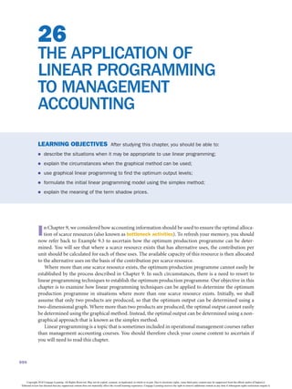
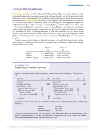
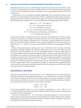
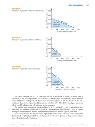
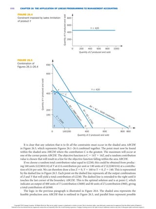
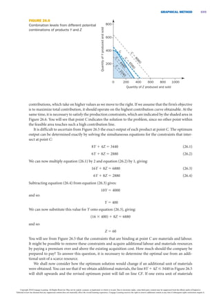
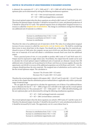
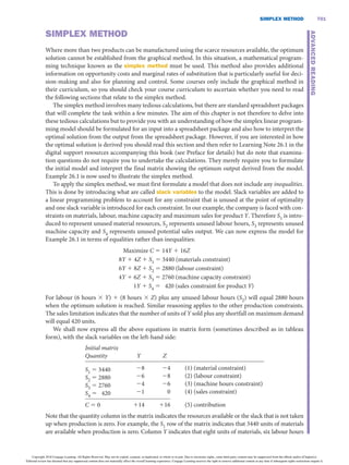
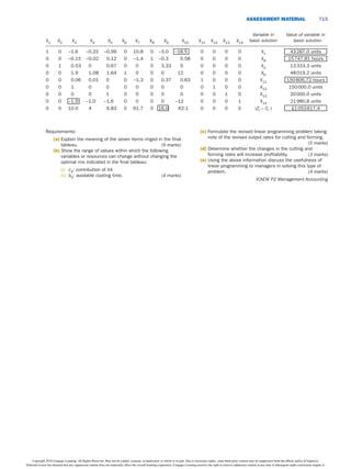
694
26
THE APPLICATION OF
LINEAR PROGRAMMING
TO MANAGEMENT
ACCOUNTING
LEARNiNG OBJECTiVES After studying this chapter, you should be able to:
● describe the situations when it may be appropriate to use linear programming;
● explain the circumstances when the graphical method can be used;
● use graphical linear programming to find the optimum output levels;
● formulate the initial linear programming model using the simplex method;
● explain the meaning of the term shadow prices.
in Chapter 9, we considered how accounting information should be used to ensure the optimal alloca-
tion of scarce resources (also known as bottleneck activities). To refresh your memory, you should
now refer back to Example 9.3 to ascertain how the optimum production programme can be deter-
mined. You will see that where a scarce resource exists that has alternative uses, the contribution per
unit should be calculated for each of these uses. The available capacity of this resource is then allocated
to the alternative uses on the basis of the contribution per scarce resource.
Where more than one scarce resource exists, the optimum production programme cannot easily be
established by the process described in Chapter 9. In such circumstances, there is a need to resort to
linear programming techniques to establish the optimum production programme. Our objective in this
chapter is to examine how linear programming techniques can be applied to determine the optimum
production programme in situations where more than one scarce resource exists. Initially, we shall
assume that only two products are produced, so that the optimum output can be determined using a
two-dimensional graph. Where more than two products are produced, the optimal output cannot easily
be determined using the graphical method. Instead, the optimal output can be determined using a non-
graphical approach that is known as the simplex method.
Linear programming is a topic that is sometimes included in operational management courses rather
than management accounting courses. You should therefore check your course content to ascertain if
you will need to read this chapter.
Copyright 2018 Cengage Learning. All Rights Reserved. May not be copied, scanned, or duplicated, in whole or in part. Due to electronic rights, some third party content may be suppressed from the eBook and/or eChapter(s).
Editorial review has deemed that any suppressed content does not materially affect the overall learning experience. Cengage Learning reserves the right to remove additional content at any time if subsequent rights restrictions require it.
LiNEAR PROGRAMMiNG 695
LiNEAR PROGRAMMiNG
Linear programming is a powerful mathematical technique that can be applied to the problem of ration-
ing limited facilities and resources among many alternative uses in such a way that the optimum benefits
can be derived from their utilization. It seeks to find a feasible combination of output that will maximize
or minimize the objective function. The objective function refers to the quantification of an objective,
and usually takes the form of maximizing profits or minimizing costs. Linear programming may be
used when relationships can be assumed to be linear and where an optimal solution does, in fact, exist.
To comply with the linearity assumption, it must be assumed that the contribution per unit for each
product and the utilization of resources per unit are the same whatever quantity of output is produced
and sold within the output range being considered. It must also be assumed that units produced and
resources allocated are infinitely divisible. This means that an optimal plan that suggests we should
produce 94.38 units is possible. However, it will be necessary to interpret the plan as a production of
94 units.
We shall now apply this technique to the problem outlined in Example 26.1, where there is a labour
restriction plus a limitation on the availability of materials and machine hours. The contributions per
scarce resource are as follows:
   
Product Y
(£)  
Product Z
(£)
Labour
Material
Machine capacity


2.33 (£14/6 hours)
1.75 (£14/8 units)
3.50 (£14/4 hours)


2.00 (£16/8 hours)
4.00 (£16/4 units)
2.67 (£16/6 hours)
The LP company currently makes two products. The standards per unit of product are as follows:
Product Y   (£)   (£)   Product Z   (£)   (£)
Product Y
Standard selling price
Less standard costs:
Materials (eight units at £4)
Labour (six hours at £10)
Variable overhead
(four machine hours at £1)
 
Contribution


32
60
4
 
110


96
14
Product Z
Standard selling price
Less standard costs:
Materials (four units at £4)
Labour (eight hours at £10)
Variable overhead
(six machine hours at £1)
 
Contribution


16
80
6
 
118


102
16
During the next accounting period, the availability of resources are expected to be subject to the following
limitations:
Labour
Materials
Machine capacity


2880 hours
3440 units
2760 hours
The marketing manager estimates that the maximum sales potential for product Y is limited to 420 units.
There is no sales limitation for product Z. You are asked to advise how these limited facilities and resources
can best be used so as to gain the optimum benefit from them.
EXAMPLE 26.1
Multiple resource constraint problem
Copyright 2018 Cengage Learning. All Rights Reserved. May not be copied, scanned, or duplicated, in whole or in part. Due to electronic rights, some third party content may be suppressed from the eBook and/or eChapter(s).
Editorial review has deemed that any suppressed content does not materially affect the overall learning experience. Cengage Learning reserves the right to remove additional content at any time if subsequent rights restrictions require it.
CHAPTER 26 THE APPLiCATiON OF LiNEAR PROGRAMMiNG TO MANAGEMENT ACCOUNTiNG
696
This analysis shows that product Y yields the largest contribution per labour hour and product Z yields
the largest contribution per unit of scarce materials, but there is no clear indication of how the quantity
of scarce resources should be allocated to each product. Linear programming should be used in such
circumstances.
The procedure is, first, to formulate the problem algebraically, with Y denoting the number of units
of product Y and Z the number of units of product Z that are manufactured by the company. Second, we
must specify the objective function, which in this example is to maximize contribution (denoted by C),
followed by the input constraints. We can now formulate the linear programming model as follows:
Maximize C 5 14Y 1 16Z subject to
8Y 1 4Z # 3440 (material constraint)
6Y 1 8Z # 2880 (labour constraint)
4Y 1 6Z # 2760 (machine capacity constraint)
0 # Y # 420 (maximum and minimum sales limitation)
Z $ 0 (minimum sales limitation)
In this model, ‘maximize C’ indicates that we wish to maximize contribution with an unknown number
of units of Y produced, each yielding a contribution of £14 per unit, and an unknown number of units
of Z produced, each yielding a contribution of £16. The labour constraint indicates that six hours of
labour are required for each unit of product Y that is made and eight hours for each unit of product Z.
Thus (6 hours 3 Y) 1 (8 hours 3 Z) cannot exceed 2880 hours. Similar reasoning applies to the other
inputs.
Because linear programming is nothing more than a mathematical tool for solving constrained
optimization problems, nothing in the technique itself ensures that an answer will ‘make sense’. For
example, in a production problem, for some very unprofitable product, the optimal output level may
be a negative quantity, which is clearly an impossible solution. To prevent such nonsensical results, we
must include a non-negativity requirement, which is a statement that all variables in the problem must
be equal to or greater than zero. We must therefore add to the model in our example the constraint that
Y and Z must be greater than or equal to zero, i.e. Z $ 0 and 0 # Y # 420. The latter expression indicates
that sales of Y cannot be less than zero or greater than 420 units. The model can be solved graphically
or by the simplex method. When no more than two products are manufactured, the graphical method
can be used, but this becomes impracticable where more than two products are involved and it is then
necessary to resort to the simplex method.
GRAPHiCAL METHOD
Taking the first constraint for the materials input 8Y 1 4Z # 3440 means that we can make a maximum
of 860 units of product Z when production of product Y is zero. The 860 units is arrived at by dividing
the 3440 units of materials by the four units of material required for each unit of product Z. Alterna-
tively, a maximum of 430 units of product Y can be made (3440 units divided by eight units of materials)
if no materials are allocated to product Z. We can therefore state that:
when Y 5 0, Z 5 860
when Z 5 0, Y 5 430
These items are plotted in Figure 26.1, with a straight line running from Z = 0, Y = 430 to Y = 0,
Z = 860. Note that the vertical axis represents the number of units of Y produced and the horizontal axis
the number of units of Z produced.
The area to the left of line 8Y 1 4Z # 3440 contains all possible solutions for Y and Z in this par-
ticular situation, and any point along the line connecting these two outputs represents the maximum
combinations of Y and Z that can be produced with not more than 3440 units of materials. Every point
to the right of the line violates the material constraint.
Copyright 2018 Cengage Learning. All Rights Reserved. May not be copied, scanned, or duplicated, in whole or in part. Due to electronic rights, some third party content may be suppressed from the eBook and/or eChapter(s).
Editorial review has deemed that any suppressed content does not materially affect the overall learning experience. Cengage Learning reserves the right to remove additional content at any time if subsequent rights restrictions require it.
GRAPHiCAL METHOD 697
The labour constraint 6Y 1 8Z # 2880 indicates that if production of product Z is zero, then a
maximum of 480 units of product Y can be produced (2880/6), and if the output of Y is zero then 360
units of Z (2880/8) can be produced. We can now draw a second line Y 5 480, Z = 0 to Y = 0, Z = 360,
and this is illustrated in Figure 26.2. The area to the left of line 6Y 1 8Z ≤ 2880 in this figure represents
all the possible solutions that will satisfy the labour constraint.
The machine input constraint is represented by Z = 0, Y = 690 and Y = 0, Z = 460, and the line
indicating this constraint is illustrated in Figure 26.3. The area to the left of the line 4Y 1 6Z ≤ 2760 in
this figure represents all the possible solutions that will satisfy the machine capacity constraint.
The final constraint is that the sales output of product Y cannot exceed 420 units. This is represented
by the line Y ≤ 420 in Figure 26.4, and all the items below this line represent all the possible solutions
that will satisfy this sales limitation.
0 200 400 600 800 1000
Quantity of Z produced and sold
800
600
400
200
Quantity
of
Y
produced
and
sold
Feasible
production
combination
8Y 1 4Z # 3440
FiGURE 26.1
Constraint imposed by limitations of materials
0 200 400 600 800 1000
Quantity of Z produced and sold
800
600
400
200
Quantity
of
Y
produced
and
sold
Feasible
production
combination
6
Y
1
8
Z
#
2
8
8
0
FiGURE 26.2
Constraint imposed by limitations of labour
0 200 400 600 800 1000
Quantity of Z produced and sold
800
600
400
200
Quantity
of
Y
produced
and
sold
Feasible
production
combination
4
Y
1
6
Z
#
2
7
6
0
FiGURE 26.3
Constraint imposed by machine capacity
Copyright 2018 Cengage Learning. All Rights Reserved. May not be copied, scanned, or duplicated, in whole or in part. Due to electronic rights, some third party content may be suppressed from the eBook and/or eChapter(s).
Editorial review has deemed that any suppressed content does not materially affect the overall learning experience. Cengage Learning reserves the right to remove additional content at any time if subsequent rights restrictions require it.
CHAPTER 26 THE APPLiCATiON OF LiNEAR PROGRAMMiNG TO MANAGEMENT ACCOUNTiNG
698
It is clear that any solution that is to fit all the constraints must occur in the shaded area ABCDE
in Figure 26.5, which represents Figures 26.1–26.4 combined together. The point must now be found
within the shaded area ABCDE where the contribution C is the greatest. The maximum will occur at
one of the corner points ABCDE. The objective function is C = 14Y 1 16Z, and a random contribution
value is chosen that will result in a line for the objective function falling within the area ABCDE.
If we choose a random total contribution value equal to £2240, this could be obtained from produc-
ing 160 units (£2240/£14) of Y at £14 contribution per unit or 140 units of Z (£2240/£16) at a contribu-
tion of £16 per unit. We can therefore draw a line Z = 0, Y = 160 to Y = 0, Z = 140. This is represented
by the dashed line in Figure 26.5. Each point on the dashed line represents all the output combinations
of Z and Y that will yield a total contribution of £2240. The dashed line is extended to the right until it
touches the last corner of the boundary ABCDE. This is the optimal solution and is at point C, which
indicates an output of 400 units of Y (contribution £5600) and 60 units of Z (contribution £960), giving
a total contribution of £6560.
The logic in the previous paragraph is illustrated in Figure 26.6. The shaded area represents the
feasible production area ABCDE that is outlined in Figure 26.5, and parallel lines represent possible
0 200 400 600 800 1000
Quantity of Z produced and sold
800
600
400
200
Quantity
of
Y
produced
and
sold
Y # 420
FiGURE 26.4
Constraint imposed by sales limitation
of product Y
0 200 400 600 800
Quantity of Z produced and sold
690
Quantity
of
Y
produced
and
sold
600
400
200
160
140 860
C
5
2
2
4
0
C
G
Y # 420
F
B
A
6
Y
1
8
Z
#
2
8
8
0
(
l
a
b
o
u
r
)
8Y 1
4Z #
3440 (materials)
4
Y
1
6
Z
#
2
7
6
0
D
E
FiGURE 26.5
Combination of
Figures 26.1–26.4
Copyright 2018 Cengage Learning. All Rights Reserved. May not be copied, scanned, or duplicated, in whole or in part. Due to electronic rights, some third party content may be suppressed from the eBook and/or eChapter(s).
Editorial review has deemed that any suppressed content does not materially affect the overall learning experience. Cengage Learning reserves the right to remove additional content at any time if subsequent rights restrictions require it.
GRAPHiCAL METHOD 699
contributions, which take on higher values as we move to the right. If we assume that the firm’s objective
is to maximize total contribution, it should operate on the highest contribution curve obtainable. At the
same time, it is necessary to satisfy the production constraints, which are indicated by the shaded area in
Figure 26.6. You will see that point C indicates the solution to the problem, since no other point within
the feasible area touches such a high contribution line.
It is difficult to ascertain from Figure 26.5 the exact output of each product at point C. The optimum
output can be determined exactly by solving the simultaneous equations for the constraints that inter-
sect at point C:
8Y 1 4Z 5 3440 (26.1)
6Y 1 8Z 5 2880 (26.2)
We can now multiply equation (26.1) by 2 and equation (26.2) by 1, giving:
16Y 1 8Z 5 6880 (26.3)
6Y 1 8Z 5 2880 (26.4)
Subtracting equation (26.4) from equation (26.3) gives:
10Y 5 4000
and so:
Y 5 400
We can now substitute this value for Y onto equation (26.3), giving:
(16 3 400) 1 8Z 5 6880
and so:
Z 5 60
You will see from Figure 26.5 that the constraints that are binding at point C are materials and labour.
It might be possible to remove these constraints and acquire additional labour and materials resources
by paying a premium over and above the existing acquisition cost. How much should the company be
prepared to pay? To answer this question, it is necessary to determine the optimal use from an addi-
tional unit of a scarce resource.
We shall now consider how the optimum solution would change if an additional unit of materials
were obtained. You can see that if we obtain additional materials, the line 8Y 1 4Z ≤ 3440 in Figure 26.5
will shift upwards and the revised optimum point will fall on line CF. If one extra unit of materials
FiGURE 26.6
Combination levels from different potential
combinations of products Y and Z
0 200 400 600 800 1000
Quantity of Z produced and sold
800
600
400
200
Quantity
of
Y
produced
and
sold
C
5
8
9
6
0
C
5
6
5
6
0
C
5
4
4
8
0
C
5
2
2
4
0
C
Copyright 2018 Cengage Learning. All Rights Reserved. May not be copied, scanned, or duplicated, in whole or in part. Due to electronic rights, some third party content may be suppressed from the eBook and/or eChapter(s).
Editorial review has deemed that any suppressed content does not materially affect the overall learning experience. Cengage Learning reserves the right to remove additional content at any time if subsequent rights restrictions require it.
CHAPTER 26 THE APPLiCATiON OF LiNEAR PROGRAMMiNG TO MANAGEMENT ACCOUNTiNG
700
is obtained, the constraints 8Y 1 4Z ≤ 3440 and 6Y 1 8Z ≤ 2880 will still be binding, and the new
optimum plan can be determined by solving the following simultaneous equations:
8Y 1 4Z 5 3441 (revised materials constraint)
6Y 1 8Z 5 2880 (unchanged labour constraint)
The revised optimal output when the above equations are solved is 400.2 units of Y and 59.85 units of Z.
Therefore the planned output of product Y should be increased by 0.2 units, and planned production of
Z should be reduced by 0.15 units. This optimal response from an independent marginal increase in a
resource is called the marginal rate of substitution. The change in contribution arising from obtaining
one additional unit of materials is as follows:
    (£)
Increase in contribution from Y (0.2 3 £14)
Decrease in contribution of Z (0.15 3 £16)
Increase in contribution


2.80
(2.40)
0.40
Therefore the value of an additional unit of materials is £0.40. The value of an independent marginal
increase of scarce resource is called the opportunity cost or shadow price. We shall be considering
these terms in more detail later in the chapter. You should note at this stage that, for materials pur-
chased in excess of 3440 units, the company can pay up to £0.40 over and above the present acquisi-
tion cost of materials of £4 and still obtain a contribution towards fixed costs from the additional
output.
From a practical point of view, it is not possible to produce 400.2 units of Y and 59.85 units of Z.
Output must be expressed in single whole units. Nevertheless, the output from the model can be used
to calculate the revised optimal output if additional units of materials are obtained. Assume that 100
additional units of materials can be purchased at £4.20 per unit from an overseas supplier. Because the
opportunity cost (£0.40) is in excess of the additional acquisition cost of £0.20 per unit (£4.20 2 £4), the
company should purchase the extra materials. The marginal rates of substitution can be used to calcu-
late the revised optimum output. The calculation is:
Increase Y by 20 units (100 3 0.2 units)
Decrease Z by 15 units (100 3 0.15 units)
Therefore the revised optimal output is 420 outputs (400 1 20) of Y and 35 units (60 2 15) of Z. You will
see later in this chapter that the substitution process outlined above is applicable only within a particular
range of material usage.
We can apply the same approach to calculate the opportunity cost of labour. If an additional labour
hour is obtained, the line 6Y 1 8Z = 2880 in Figure 26.5 will shift to the right and the revised optimal
point will fall on line CG. The constraints 8Y 1 4Z = 3440 and 6Y 1 8Z = 2880 will still be binding, and
the new optimum plan can be determined by solving the following simultaneous equations:
8Y 1 4Z 5 3440 (unchanged materials constraint)
6Y 1 8Z 5 2881 (revised labour constraint)
The revised optimal output when the above equations are solved is 399.9 units of Y and 60.2 units of Z.
Therefore the planned output of product Y should be decreased by 0.1 units and planned production of
Z should be increased by 0.2 units. The opportunity cost of a scarce labour hour is:
    (£)
Decrease in contribution from Y (0.1 3 £14)
Increase in contribution from Z (0.2 3 £16)
Increase in contribution (opportunity cost)


(1.40)
3.20
1.80
Copyright 2018 Cengage Learning. All Rights Reserved. May not be copied, scanned, or duplicated, in whole or in part. Due to electronic rights, some third party content may be suppressed from the eBook and/or eChapter(s).
Editorial review has deemed that any suppressed content does not materially affect the overall learning experience. Cengage Learning reserves the right to remove additional content at any time if subsequent rights restrictions require it.
SiMPLEX METHOD 701
SiMPLEX METHOD
Where more than two products can be manufactured using the scarce resources available, the optimum
solution cannot be established from the graphical method. In this situation, a mathematical program-
ming technique known as the simplex method must be used. This method also provides additional
information on opportunity costs and marginal rates of substitution that is particularly useful for deci-
sion-making and also for planning and control. Some courses only include the graphical method in
their curriculum, so you should check your course curriculum to ascertain whether you need to read
the following sections that relate to the simplex method.
The simplex method involves many tedious calculations, but there are standard spreadsheet packages
that will complete the task within a few minutes. The aim of this chapter is not therefore to delve into
these tedious calculations but to provide you with an understanding of how the simplex linear program-
ming model should be formulated for an input into a spreadsheet package and also how to interpret the
optimal solution from the output from the spreadsheet package. However, if you are interested in how
the optimal solution is derived you should read this section and then refer to Learning Note 26.1 in the
digital support resources accompanying this book (see Preface for details) but do note that examina-
tion questions do not require you to undertake the calculations. They merely require you to formulate
the initial model and interpret the final matrix showing the optimum output derived from the model.
Example 26.1 is now used to illustrate the simplex method.
To apply the simplex method, we must first formulate a model that does not include any inequalities.
This is done by introducing what are called slack variables to the model. Slack variables are added to
a linear programming problem to account for any constraint that is unused at the point of optimality
and one slack variable is introduced for each constraint. In our example, the company is faced with con-
straints on materials, labour, machine capacity and maximum sales for product Y. Therefore S1 is intro-
duced to represent unused material resources, S2 represents unused labour hours, S3 represents unused
machine capacity and S4 represents unused potential sales output. We can now express the model for
Example 26.1 in terms of equalities rather than inequalities:
Maximize C 5 14Y 1 16Z
8Y 1 4Z 1 S1 5 3440 (materials constraint)
6Y 1 8Z 1 S2 5 2880 (labour constraint)
4Y 1 6Z 1 S3 5 2760 (machine capacity constraint)
1Y 1 S4 5 420 (sales constraint for product Y)
For labour (6 hours 3 Y) 1 (8 hours 3 Z) plus any unused labour hours (S2) will equal 2880 hours
when the optimum solution is reached. Similar reasoning applies to the other production constraints.
The sales limitation indicates that the number of units of Y sold plus any shortfall on maximum demand
will equal 420 units.
We shall now express all the above equations in matrix form (sometimes described as in tableau
form), with the slack variables on the left-hand side:
Initial matrix
Quantity
 
Y
 
Z
   
S1 = 3440
S2 = 2880
S3 = 2760
S4 = 420


28
26
24
21


24
28
26
0


(1) (material constraint)
(2) (labour constraint)
(3) (machine hours constraint)
(4) (sales constraint)
C = 0   114   116  (5) contribution
Note that the quantity column in the matrix indicates the resources available or the slack that is not taken
up when production is zero. For example, the S1 row of the matrix indicates that 3440 units of materials
are available when production is zero. Column Y indicates that eight units of materials, six labour hours
ADVANCED
READiNG
Copyright 2018 Cengage Learning. All Rights Reserved. May not be copied, scanned, or duplicated, in whole or in part. Due to electronic rights, some third party content may be suppressed from the eBook and/or eChapter(s).
Editorial review has deemed that any suppressed content does not materially affect the overall learning experience. Cengage Learning reserves the right to remove additional content at any time if subsequent rights restrictions require it.
CHAPTER 26 THE APPLiCATiON OF LiNEAR PROGRAMMiNG TO MANAGEMENT ACCOUNTiNG
702
and four machine hours are required to produce one unit of product Y and this will reduce the potential
sales of Y by one. You will also see from column Y that the production of one unit of Y will yield £14
contribution. Similar reasoning applies to column Z. Note that the entry in the contribution row (i.e. the
C row) for the quantity column is zero because this first matrix is based on nil production, which gives a
contribution of zero.
The simplex method involves the application of matrix algebra to generate a series of matrices until
a final matrix emerges that represents the optimal solution based on the initial model. Learning Note
26.1 explains how the final matrix is derived (see the digital resources). The final matrix containing the
optimal solution is shown below:
Final matrix
Quantity
 
S1
 
S2
   
Y = 400
Z = 60
S3 = 800
S4 = 20


21
∙5
13
∙20
21
∙10
11
∙5


11∙10
21
∙5
14∙5
21∙10


(1)
(2)
(3)
(4)
C = 6560   22∙5   214∙5   (5)
Interpreting the final matrix
The final matrix can be interpreted using the same approach that was used for the initial matrix but
the interpretation is more complex. The contribution row (equation 5) of the final matrix contains
only negative items, which signifies that the optimal solution has been reached. The quantity column
for any products listed on the left-hand side of the matrix indicates the number of units of the prod-
uct that should be manufactured when the optimum solution is reached. 400 units of Y and 60 units
of Z should therefore be produced, giving a total contribution of £6560. This agrees with the results
we obtained using the graphical method. When an equation appears for a slack variable, this indicates
that unused resources exist. The final matrix therefore indicates that the optimal plan will result in 800
unused machine hours (S3) and an unused sales potential of 20 units for product Y (S4). The fact that
there is no equation for S1 and S2 means that these are the inputs that are fully utilized and that limit
further increases in output and profit.
The S1 column (materials) of the final matrix indicates that the materials are fully utilized. (Whenever
resources appear as column headings in the final matrix, this indicates that they are fully utilized.) So, to
obtain a unit of materials, the column for S1 indicates that we must alter the optimum production pro-
gramme by increasing production of product Z by 3
∙20 of a unit and decreasing production of product Y by
1
∙5 of a unit. The effect of removing one scarce unit of material from the production process is summarized
in Exhibit 26.1.
EXHiBiT 26.1 The effect of removing one unit of material from the optimum production programme
S3 S4 S1 S2
    Machine capacity   Sales of Y Materials Labour  
Contribution
(£)
Increase
product Z by
3
∙
20 of a unit
 
29
∙
10(3
∙
20 3 6)
 
— 23
∙
5(3
∙
20 3 4) –11
∙
5(3
∙
20 3 8)
 
+22
∙
5(3
∙
20 3 16)
Decrease
product Y by
1
∙
5 of a unit
 
+4
∙5(1
∙
5 3 4)
 
+1
∙
5 +13
∙
5(1
∙
5 3 8) +11
∙
5(1
∙
5 3 6)
 
–24
∙
5(1
∙
5 3 14)
Net effect 21
∙
10 +1
∙
5 +1 Nil –2
∙
5
Copyright 2018 Cengage Learning. All Rights Reserved. May not be copied, scanned, or duplicated, in whole or in part. Due to electronic rights, some third party content may be suppressed from the eBook and/or eChapter(s).
Editorial review has deemed that any suppressed content does not materially affect the overall learning experience. Cengage Learning reserves the right to remove additional content at any time if subsequent rights restrictions require it.
SiMPLEX METHOD 703
Look at the machine capacity column of Exhibit 26.1. If we increase production of product Z by 3∙20 of
a unit then more machine hours will be required, leading to the available capacity being reduced by 9∙10
of an hour. Each unit of product Z requires six machine hours, so 3
∙20 of a unit will require 9∙10 of an hour
(3
∙20 3 6). Decreasing production of product Y by 1∙5 unit will release 4∙5 of a machine hour, given that one
unit of product Y requires four machine hours. The overall effect of this process is to reduce the available
machine capacity by 1∙10 of a machine hour. Similar principles apply to the other calculations presented
in Exhibit 26.1.
WeshallnowreconciletheinformationsetoutinExhibit26.1withthematerialscolumn(S1)ofthefinal
matrix. The S1 column of the final matrix indicates that, to release one unit of materials from the optimum
production programme, we should increase the output of product Z by 3
∙20 and decrease product Y by 1∙5
of a unit. This substitution process will lead to the unused machine capacity being reduced by 1∙10 of a
machine hour, an increase in the unfulfilled sales demand of product Y (S4) by 1
∙5 of a unit and a reduction
incontributionof£2∙5.AllthisinformationisobtainedfromcolumnS1 ofthefinalmatrix,andExhibit26.1
provides the proof. Note that Exhibit 26.1 also proves that the substitution process that is required to
obtain an additional unit of materials releases exactly one unit. In addition, Exhibit 26.1 indicates that
the substitution process for labour gives a net effect of zero, and so no entries appear in the S1 column of
the final matrix in respect of the labour row (i.e. S2).
The contribution row of the final matrix contains some vital information for the accountant. The
figures in this row represent opportunity costs (also known as shadow prices) for the scarce factors of
materials and labour. For example, the reduction in contribution from the loss of one unit of materials is
£2∙5 (£0.40) and from the loss of one labour hour is £14∙5 (£1.80). Our earlier studies have indicated that
this information is vital for decision-making and we shall use this information again shortly to establish
the relevant costs of the resources.
The proof of the opportunity costs can be found in Exhibit 26.1. From the contribution column we
can see that the loss of one unit of materials leads to a loss of contribution of £0.40.
Substitution process when additional resources are obtained
Management may be able to act to remove a constraint that is imposed by the shortage of a scarce
resource. For example, the company might obtain substitute materials or it may purchase the materi-
als from an overseas supplier. A situation may therefore occur where resources additional to those
included in the model used to derive the optimum solution are available. In such circumstances,
the marginal rates of substitution specified in the final matrix can indicate the optimum use of the
additional resources. However, when additional resources are available it is necessary to reverse the
signs in the final matrix. The reason is that the removal of one unit of materials from the optimum
production programme requires that product Z be increased by 3
∙20 of a unit and product Y decreased
by 1
∙5 of a unit.
If we then decide to return released materials to the optimum production programme, we must
reverse this process – that is, increase product Y by 1
∙5 of a unit and reduce product Z by 3
∙20 of a
unit. The important point to remember is that when considering the response to obtaining additional
resources over and above those specified in the initial model, the signs of all the items in the final matrix
must be reversed.
We can now establish how we should best use an additional unit of scarce materials. Inspection of
the final matrix indicates that product Y should be increased by 1
∙5 of a unit and product Z reduced by
3
∙20, giving an additional contribution of £0.40. Note that this is identical with the solution we obtained
using the graphical method.
Note that this process will lead to an increase in machine hours of 1
∙10 hour (S3) and a decrease in
potential sales of product Y by 1
∙5 (S4). Similarly, if we were to obtain an additional labour hour, we
should increase production of Z by 1
∙5 of a unit and decrease production of product Y by 1
∙10 of a unit,
which would yield an additional contribution of £1.80. These are the most efficient uses that can be
obtained from additional labour and material resources. From a practical point of view, decisions will
Copyright 2018 Cengage Learning. All Rights Reserved. May not be copied, scanned, or duplicated, in whole or in part. Due to electronic rights, some third party content may be suppressed from the eBook and/or eChapter(s).
Editorial review has deemed that any suppressed content does not materially affect the overall learning experience. Cengage Learning reserves the right to remove additional content at any time if subsequent rights restrictions require it.
CHAPTER 26 THE APPLiCATiON OF LiNEAR PROGRAMMiNG TO MANAGEMENT ACCOUNTiNG
704
not involve the use of fractions; for example, the LP company considered here might be able to obtain
200 additional labour hours; the final matrix indicates that optimal production plan should be altered by
increasing production of product Z by 40 units (200 3 1
∙5 of a unit) and decreasing production of prod-
uct Y by 20 units. This process will lead to machine capacity being reduced by 160 hours and potential
sales of product Y being increased by 20 units.
It is possible that examination questions may present the final matrix in a different format to the
approach illustrated in this chapter. You should refer to the Key examination points section at the end of
the chapter for an explanation of how you can reconcile the alternative approaches.
USES OF LiNEAR PROGRAMMiNG
Calculation of relevant costs
The calculation of relevant costs is essential for decision-making. When a resource is scarce, alternative
uses exist that provide a contribution. An opportunity cost is therefore incurred whenever the resource
is used. The relevant cost for a scarce resource is calculated as:
acquisition cost of resource 1 opportunity cost
When more than one scarce resource exists, the opportunity cost should be established using linear
programming techniques. Note that the opportunity costs of materials and labour are derived from the
Uses of linear programming – linear
programming in the supply chain
SAP
, the global leader in enterprise resource plan-
ning (ERP) systems, offers several tools to help a
business find an optimal solution to scheduling
and planning problems. The advanced planner and
optimizer (APO) offers solutions to help firms find
the best and most cost-effective solution in areas
like demand planning, production planning, trans-
portation planning and supply network planning.
The later module, supply network planning (SNP)
allows planners to determine optimal production
plans, distribution plans and purchasing plans.
According to SAP’s documentation, the SNP mod-
ule offer an optimizer that will obtain the most cost-
effective solution based on the following criteria:
● production, procurement, storage and
transportation costs;
● costs for increasing the production capacity,
storage capacity, transportation capacity and
handling capacity;
● costs for violating (falling below) the safety
stock level;
● costs for late delivery;
● stock-out costs.
The optimizer uses linear programming method
to take account of all planning factors simultane-
ously. According to SAP’s documentation, as more
constraints are activated, the optimization problem
becomes more complex and takes more time to
complete. The SNP module offers several variants
on linear programming to allow maximum applica-
bility to varying problem scenarios.
Questions
1 Can you think of factors that might affect
production, procurement, storage or
transportation costs as referred to above?
2 Given the apparently large number of
factors taken into account by the optimizer
in SNP
, do you think the business and/or the
system can run the optimizer programme
frequently?
Reference
help.sap.com/saphelp_scm41/helpdata/en/09/707b37
db6bcd66e10000009b38f889/content.htm
REAL WORLD
ViEWS 26.1
Copyright 2018 Cengage Learning. All Rights Reserved. May not be copied, scanned, or duplicated, in whole or in part. Due to electronic rights, some third party content may be suppressed from the eBook and/or eChapter(s).
Editorial review has deemed that any suppressed content does not materially affect the overall learning experience. Cengage Learning reserves the right to remove additional content at any time if subsequent rights restrictions require it.
USES OF LiNEAR PROGRAMMiNG 705
final row (monetary figures expressed in fractions) of the third and final matrix. Let us now calculate
the relevant costs for the resources used by the LP company. The costs are as follows:
materials 5 £4.40 (£4 acquisition cost plus £0.40 opportunity cost)
labour 5 £11.80 (£10 acquisition cost plus £1.80 opportunity cost)
variable overheads 5 £1.00 (£1 acquisition cost plus zero opportunity cost)
fixed overheads 5 nil
Because variable overheads are assumed to vary in proportion to machine hours, and because machine
hours are not scarce, no opportunity costs arise for variable overheads. Fixed overheads have not been
included in the model, since they do not vary in the short term with changes in activity. The relevant
cost for fixed overheads is therefore zero.
Selling different products
We shall now assume that the company is contemplating selling a modified version of product Y (called
product L) in a new market. The market price is £160 and the product requires ten units input of each
resource. Should this product L be manufactured? Conventional accounting information does not provide
us with the information necessary to make this decision. Product L can be made only by restricting output
of Y and Z, because of the input constraints, and we need to know the opportunity costs of releasing
the scarce resources to this new product. Opportunity costs were incorporated in our calculation of the
relevant costs for each of the resources, and so the relevant information for the decision is as follows:
    (£)   (£)
Selling price of product L
Less relevant costs:
Materials (10 3 4.40)
Labour (10 3 11.80)
Variable overhead (10 3 1.00)
Contribution


44
118
10


160


172
      (–12)
Total planned contribution will be reduced by £12 for each unit produced of product L.
Maximum payment for additional scarce resources
Opportunity costs provide important information in situations where a company can obtain additional
scarce resources, but only at a premium. How much should the company be prepared to pay? For example,
the company may be able to remove the labour constraint by paying overtime. The final matrix indicates
that the company can pay up to an additional £1.80 over and above the standard wage rate for each hour
worked in excess of 2880 hours and still obtain a contribution from the use of this labour hour. The total
contribution will therefore be improved by any additional payment below £1.80 per hour. Similarly, LP
will improve the total contribution by paying up to £0.40 in excess of the standard material cost for units
obtained in excess of 3440 units. Hence the company will increase short-term profits by paying up to
£11.80 for each additional labour hour in excess of 2880 hours and up to £4.40 for units of material that
are acquired in excess of 3440 units.
Control
Opportunity costs are also important for cost control. For example, material wastage is reflected in an
adverse material usage variance. The responsibility centre should therefore be identified not only with the
Copyright 2018 Cengage Learning. All Rights Reserved. May not be copied, scanned, or duplicated, in whole or in part. Due to electronic rights, some third party content may be suppressed from the eBook and/or eChapter(s).
Editorial review has deemed that any suppressed content does not materially affect the overall learning experience. Cengage Learning reserves the right to remove additional content at any time if subsequent rights restrictions require it.
CHAPTER 26 THE APPLiCATiON OF LiNEAR PROGRAMMiNG TO MANAGEMENT ACCOUNTiNG
706
acquisition cost of £4 per unit but also with the opportunity cost of £0.40 from the loss of one scarce unit of
materials. This process highlights the true cost of the inefficient usage of scarce resources and encourages
responsibility heads to pay special attention to the control of scarce factors of production. This approach is
particularly appropriate where a firm has adopted an optimized production technology (OPT) strategy (see
Chapter 9) because variance arising from bottleneck operations will be reported in terms of opportunity cost
rather than acquisition cost.
Managing constraints
When scarce resources are fully utilized they are referred to as bottleneck operations/resources. It is
important that managers seek to increase the efficiency and capacity of bottleneck operations. Capac-
ity can be increased by working overtime on the bottleneck, subcontracting some of the work that is
undertaken by bottleneck operations, investing in additional capacity at the bottleneck and implement-
ing business process improvements such as business process engineering and total quality management
processes described in Chapter 22.
Capital budgeting
Linear programming can be used to determine the optimal investment programme when capital ration-
ing exists. This topic tends not to form part of the management accounting curriculum for most courses.
You should refer to Learning Note 26.2 (see the digital resources) if you wish to study how linear pro-
gramming can be used in capital investment appraisal.
Sensitivity analysis
Opportunity costs are of vital importance in making management decisions, but production con-
straints do not exist permanently, and therefore opportunity costs cannot be regarded as perma-
nent. There is a need to ascertain the range over which the opportunity cost applies for each input.
This information can be obtained from the final matrix. For materials, we merely examine the
negative items for column S1 in the final matrix and divide each item into the quantity column as
follows:
Y 5 400∙(21∙5) 5 22000
S3 5 800∙(21∙10) 5 28000
The number closest to zero in this calculation (namely 22000) indicates by how much the avail-
ability of materials used in the model can be reduced. Given that the model was established using
3440 units of materials, the lower limit of the range is 1440 units (3440 2 2000). The upper limit
is determined in a similar way. We divide the positive items in column S4 into the quantity column
as follows:
Z 5 60∙3∙20 5 400
S4 5 20∙ 1∙5 5 100
The lower number in the calculation (namely 100) indicates by how much the materials can be increased.
Adding this to the 3440 units of materials indicates that the upper limit of the range is 3540 units. The
opportunity cost and marginal rates of substitution for materials therefore apply over the range of 1440 to
3540 units.
We shall now consider the logic on which these calculations are based. The lower limit is determined
by removing materials from the optimum production programme. We have previously established from
the final matrix and Exhibit 26.1 that removing one unit of material from the optimum production
programme means that product Y will be reduced by 1
∙5 and machine capacity will be reduced by 1
∙10 of
Copyright 2018 Cengage Learning. All Rights Reserved. May not be copied, scanned, or duplicated, in whole or in part. Due to electronic rights, some third party content may be suppressed from the eBook and/or eChapter(s).
Editorial review has deemed that any suppressed content does not materially affect the overall learning experience. Cengage Learning reserves the right to remove additional content at any time if subsequent rights restrictions require it.
707
SUMMARY
an hour. Since the final matrix indicates an output of 400 units of product Y, this reduction can only be
carried out 2000 times (400/1
∙5) before the process must stop. Similarly, 800 hours of machine capacity
are still unused, and the reduction process can only be carried out 8000 times (800/1
∙10) before the pro-
cess must stop. Given the two constraints on reducing materials, the first constraint that is reached is the
reduction of product Y. The planned usage of materials can therefore be reduced by 2000 units before
the substitution process must stop. The same reasoning applies (with the signs reversed) in understand-
ing the principles for establishing the upper limit of the range.
Similar reasoning can be applied to establish that the opportunity cost and marginal rates of sub-
stitution apply for labour hours over a range of 2680 to 3880 hours. For any decisions based on scarce
inputs outside the ranges specified a revised model must be formulated and a revised final matrix
produced. From this matrix, revised opportunity costs and marginal rates of substitution can be
established.
SUMMARY
The following items relate to the learning objectives listed at the beginning of the chapter.
● Describe the situations when it may be appropriate to use linear programming.
Conventional limiting factor analysis (see Chapter 9) should be used when there is only one
scarce factor. Linear programming can be used to determine the production programme that
maximizes total contribution when there is more than one scarce input factor.
● Explain the circumstances when the graphical method can be used.
The graphical method can be used with two products. Where more than two products are involved,
the simplex method should be used.
● Use graphical linear programming to find the optimum output levels.
Production/sales quantities for one of the two products are labelled on the horizontal axis and the
vertical axis is used for the other product. Combinations of the maximum output (based on the
two products) from fully utilizing each resource, and any sales volume limitations, are plotted on
the graph. A series of contribution lines are plotted based on the potential output levels for each
product that will achieve a selected total contribution. The optimum output levels are derived at
the point where the feasible production region touches the highest contribution line. The process
is illustrated in Figure 26.5 using the data presented in Example 26.1.
● Formulate the initial linear programming model using the simplex method.
Assuming that the objective function is to maximize total contribution, the objective function
should initially be specified expressed in terms of the contributions per unit for each product.
Next, the constraints should be listed in equation form with slack variables introduced to ensure
that model is specified in terms of equalities rather than inequalities. The initial matrix is pre-
pared by converting the linear programming model into a matrix format. The process is illustrated
using Example 26.1.
● Explain the meaning of the term shadow prices.
The simplex method of linear programming generates shadow prices (also known as opportunity
costs) for each of those scarce resources that are fully utilized in the optimum production pro-
gramme. The shadow prices represent the reduction in total contribution that will occur from the
loss of one unit of a scarce resource. Conversely, they represent the increase in total contribution
that will occur if an additional unit of the scarce resource can be obtained.
Copyright 2018 Cengage Learning. All Rights Reserved. May not be copied, scanned, or duplicated, in whole or in part. Due to electronic rights, some third party content may be suppressed from the eBook and/or eChapter(s).
Editorial review has deemed that any suppressed content does not materially affect the overall learning experience. Cengage Learning reserves the right to remove additional content at any time if subsequent rights restrictions require it.
CHAPTER 26 THE APPLiCATiON OF LiNEAR PROGRAMMiNG TO MANAGEMENT ACCOUNTiNG
708
KEY TERMS AND CONCEPTS
Bottleneck activities Activities or operations where
constraints apply arising from demand exceeding
available capacity.
Bottleneck operations/resources Scarce resources
that are fully utilized and therefore can present
limiting factors.
Linear programming A mathematical technique used
to determine how to employ limited resources to
achieve optimum benefits.
Marginal rate of substitution The optimal response
from an independent marginal increase in a resource.
Objective function In linear programming, the
objective to be minimized or maximized.
Opportunity cost The value of an independent
marginal increase of a scarce resource, also known
as the shadow price.
Shadow price The value of an independent marginal
increase of a scarce resource, also known as the
opportunity cost.
Simplex method A mathematical technique used
in linear programming to solve optimization
problems.
Slack variable A variable that is added to a linear
programming problem to account for any constraint
that is unused at the point of optimality and so
turn an inequality into an equality.
KEY EXAMiNATiON POiNTS
A common error is to state the objective function in
terms of profit per unit. This is incorrect, because the
fixed cost per unit is not constant. The objective function
should be expressed in terms of contribution per unit.
You should note that there are several ways of formulat-
ing the matrices for a linear programming model. The
approach adopted in this chapter was to formulate the
first matrix with positive contribution signs and negative
signs for the slack variable equations. The optimal solu-
tion occurs when the signs in the contribution row are
all negative. Sometimes examination questions are set
that adopt the opposite procedure. That is, the signs are
the reverse of the approach presented in this chapter.
For an illustration of this approach, see review prob-
lem IM 26.7. A more recent approach is to present
the output from the model as a computer printout. You
should refer to the solution to review problem 26.15 to
make sure you understand this approach.
Most examination questions include the final matrix
and require you to interpret the figures. You may also
be required to formulate the initial model. It is most
unlikely that you will be required to complete the cal-
culations and prepare the final matrix. However, you
may be asked to construct a graph and calculate the
marginal rates of substitution and opportunity costs.
ASSESSMENT MATERiAL
The review questions are short questions that enable you to assess your understanding of the main topics
included in the chapter. The numbers in parentheses provide you with the page numbers to refer to if you
cannot answer a specific question.
The review problems are more complex and require you to relate and apply the content to various business
problems. The problems are graded by their level of difficulty. Solutions to review problems that are not preceded
by the term ‘IM’ are provided in a separate section at the end of the book. Solutions to problems preceded by
the term ‘IM’ are provided in the Instructor’s Manual accompanying this book that can be downloaded from the
lecturer’s digital support resources. Additional review problems with fully worked solutions are provided in the
Student Manual that accompanies this book.
REVIEW QUESTIONS
26.1 Describe the situations when it may be appropriate to
use linear programming. (pp. 694–695)
26.2 Explain what is meant by the term ‘objective function’.
(p. 695)
26.3 What is the feasible production area? (p. 698)
26.4 What is the marginal rate of substitution? (p. 700)
26.5 Explain what is meant by the term ‘shadow price’.
(p. 700)
26.6 Explain the circumstances when it is appropriate to use
the simplex method. (p. 701)
26.7 What are slack variables? (p. 701)
26.8 Provide illustrations of how the information derived
from linear programming can be applied to a variety of
management accounting problems. (pp. 704–706)
26.9 Explain how sensitivity analysis can be applied to the
output of a linear programming model. (p. 706)
Copyright 2018 Cengage Learning. All Rights Reserved. May not be copied, scanned, or duplicated, in whole or in part. Due to electronic rights, some third party content may be suppressed from the eBook and/or eChapter(s).
Editorial review has deemed that any suppressed content does not materially affect the overall learning experience. Cengage Learning reserves the right to remove additional content at any time if subsequent rights restrictions require it.
ASSESSMENT MATERiAL 709
REVIEW PROBLEMS
26.10 Intermediate. Taree Limited uses linear programming
to establish the optimal production plan for the production of
its two products, A and U, given that it has the objective of
minimizing costs. The following graph has been established
bearing in mind the various constraints of the business. The
clear area indicates the feasible region.
A units
U units
C
D
B
A
E
Which points are most likely to give the optimal solution?
(a) A and B only
(b) A, B and C only
(c) D and E only
(d) B, D and E only. (2 marks)
ACCA – Financial Information for Management
26.11 Advanced: Optimal output and calculation of maximum
amount to pay for a scarce resource using the graphical
approach. THS produces two products from different combinations
of the same resource. Details of the products are shown below:
E R
per unit per unit
Selling price $ 99 $159
Material A ($2 per kg) 3kgs 2kgs
Material B ($6 per kg) 4kgs 3kgs
Machining ($7 per hour) 2 hours 3 hours
Skilled labour ($10 per hour) 2 hours 5 hours
Maximum monthly demand (units) unlimited 1500
THS is preparing the production plan for next month. The
maximum resource availability for the month is:
Material A 5000kgs
Material B 5400kgs
Machining 3000 hours
Skilled labour 4500 hours
Required:
(a) Identify, using graphical linear programming, the optimal
production plan for products E and R to maximize THS’s
profit in the month. (13 marks)
The production manager has now been able to source extra
resources:
● An employment agency would supply skilled labour for a
monthly fee of $1000 and $14 per hour worked;
● A machine that has the same variable running costs per
hour as the current machinery can be leased. The leased
machine would be able to run for 2000 hours per month.
Required:
(b) Calculate the maximum amount that should be paid
next month to lease the machine. (Note: you should
assume that a contract has already been signed with the
employment agency.) (8 marks)
(c) Explain TWO major factors that should be considered
before deciding to lease the machine. (Note: you should
assume that the data supplied are totally accurate.)
(4 marks)
CIMA P2 Performance Management
26.12 Advanced: Optimal output and calculation of shadow
prices using the graphical approach. The Cosmetic Co. is a
company producing a variety of cosmetic creams and lotions.
The creams and lotions are sold to a variety of retailers at
a price of $23.20 for each jar of face cream and $16.80
for each bottle of body lotion. Each of the products has a
variety of ingredients, with the key ones being silk powder,
silk amino acids and aloe vera. Six months ago, silk worms
were attacked by disease causing a huge reduction in the
availability of silk powder and silk amino acids. The Cosmetic
Co. had to dramatically reduce production and make part of
its workforce, which it had trained over a number of years,
redundant.
The company now wants to increase production again
by ensuring that it uses the limited ingredients available to
maximize profits by selling the optimum mix of creams and
lotions. Due to the redundancies made earlier in the year,
supply of skilled labour is now limited in the short term to 160
hours (9600 minutes) per week, although unskilled labour is
unlimited. The purchasing manager is confident that they can
obtain 5000 grams of silk powder and 1600 grams of silk amino
acids per week. All other ingredients are unlimited. The following
information is available for the two products:
Cream Lotion
Materials required: silk powder (at
$2.20 per gram)
3 grams 2 grams
– silk amino acids (at $0.80 per gram) 1 gram 0.5 grams
– aloe vera (at $1.40 per gram) 4 grams 2 grams
Labour required: skilled ($12 per hour) 4 minutes 5 minutes
– unskilled (at $8 per hour) 3 minutes 1.5 minutes
Each jar of cream sold generates a contribution of $9 per unit,
whilst each bottle of lotion generates a contribution of $8 per
unit. The maximum demand for lotions is 2000 bottles per week,
although demand for creams is unlimited. Fixed costs total
$1800 per week. The company does not keep inventory although
if a product is partially complete at the end of one week, its
production will be completed in the following week.
Required:
(a) On the graph paper provided, use linear programming
to calculate the optimum number of each product that
the Cosmetic Co. should make per week, assuming that
it wishes to maximize contribution. Calculate the total
contribution per week for the new production plan. All
workings MUST be rounded to two decimal places.
(14 marks)
(b) Calculate the shadow price for silk powder and the slack
for silk amino acids. All workings MUST be rounded to
two decimal places. (6 marks)
ACCA F5 Performance Management
26.13 Advanced: Determination of optimum production
plan using simultaneous equations (not using a graphical
approach). PTP produces two products from different
Copyright 2018 Cengage Learning. All Rights Reserved. May not be copied, scanned, or duplicated, in whole or in part. Due to electronic rights, some third party content may be suppressed from the eBook and/or eChapter(s).
Editorial review has deemed that any suppressed content does not materially affect the overall learning experience. Cengage Learning reserves the right to remove additional content at any time if subsequent rights restrictions require it.
CHAPTER 26 THE APPLiCATiON OF LiNEAR PROGRAMMiNG TO MANAGEMENT ACCOUNTiNG
710
combinations of the same resources. Details of the selling price
and costs per unit for each product are shown below:
Product E Product M
$ $
Selling price 175 125
Material A ($12 per kg) 60 24
Material B ($5 per kg) 10 15
Labour ($20 per hour) 40 20
Variable overhead
($7 per machine hour)
14 28
The fixed costs of the company are $50000 per month.
PTP aims to maximize profits from production and sales. The
production plan for June is currently under consideration.
The following resources are available in June:
Material A 4800kg
Material B 3900kg
Labour 2500 hours
Machine hours 5000 hours
Required:
(a) (i) Identify the objective function and the constraints to
be used in a linear programming model to determine
the optimum production plan for June. (3 marks)
The solution to the linear programming model shows
that the only binding constraints in June are those for
Material A and Material B.
(ii) Produce, using simultaneous equations, the optimum
production plan and resulting profit for June. (You are
NOT required to draw or sketch a graph.) (5 marks)
Based on the optimal production plan for June, the
management accountant at PTP has determined that
the shadow price for Material A is $7 per kg.
(b) Explain the meaning of the shadow price for Material A.
(2 marks)
26.14 Advanced: Optimum production programme and
interpretation of the solution of a linear programming model.
LM produces two products from different quantities of the same
resources using a just-in-time (JIT) production system. The
selling price and resource requirements of each of these two
products are as follows:
Product   L   M
Unit selling price ($)   70   90
Variable costs per unit:        
Direct labour ($7 per hour)   28   14
Direct material ($5 per kg)   10   45
Machine hours ($10 per hour)   10   20
Fixed overheads absorbed   12   6
Profit per unit   10   5
Fixed overheads are absorbed at the rate of $3 per direct
labour hour.
Market research shows that the maximum demand for
products L and M during December will be 400 units and 700
units respectively.
At a recent meeting of the purchasing and production
managers to discuss the company’s production plans for
December, the following resource availability for December
was identified:
Direct labour   3500 hours
Direct material   6000kg
Machine hours   2000 hours
Required:
(a) Prepare calculations to show, from a financial
perspective, the optimum production plan for December
and the contribution that would result from adopting
your plan. (6 marks)
(b) You have now presented your optimum plan to the
purchasing and production managers of LM. During the
presentation, the following additional information became
available:
(i) The company has agreed to an order for 250 units
of product M For a selling price of $90 per unit from
a new overseas customer. This order is in addition
to the maximum demand that was previously
predicted and must be produced and delivered in
December;
(ii) The originally predicted resource restrictions were
optimistic. The managers now agree that the
availability of all resources will be 20 per cent lower
than their original predictions.
Required:
Construct the revised resource constraints and the objective
function to be used to identify, given the additional information
above, the revised optimum production plan for December.
(6 marks)
(c) The resource constraints and objective function
requested in part (b) above have now been processed in
a simplex linear programming model and the following
solution has been printed:
Product L   400  Product L other value   0
Product M   194  Product M other vaIue   506
Direct labour   312       
Direct material ($)   1.22       
Machine hours   312       
Contribution ($)   10934.00   
Required:
Analyse the meaning of each of the above eight values in the
solution to the problem. Your answer should include a proof of
the last five of the individual values listed. (13 marks)
CIMA P5 Performance Management
26.15 Advanced: Interpretation of the linear programming
solution. Woodalt plc has two automated machine groups X
and Y, through which timber is passed in order to produce two
models of an item of sports equipment. The models are called
‘Traditional’ and ‘Hightech’.
The following forecast information is available for the year to
31 December:
  ‘Traditional’   ‘Hightech’
(i) Maximum sales potential (units)   6000   10000
(ii) Equipment unit data:        
Selling price   £100   £90
Machine time: group X (hours)   0.5   0.3
group Y (hours)   0.4   0.45
(iii) Machine groups X and Y have maximum operating hours
of 3400 and 3840, respectively. The sports equipment
production is the sole use available for the production
capacity.
(iv) The maximum quantity of timber available is 34000 metres.
Each product unit requires four metres of timber. Timber
may be purchased in lengths as required at £5 per metre.
(v) Variable machine overhead cost for machine groups
X and Y is estimated at £25 and £30 per machine hour,
respectively.
(vi) All units are sold in the year in which they are produced.
Copyright 2018 Cengage Learning. All Rights Reserved. May not be copied, scanned, or duplicated, in whole or in part. Due to electronic rights, some third party content may be suppressed from the eBook and/or eChapter(s).
Editorial review has deemed that any suppressed content does not materially affect the overall learning experience. Cengage Learning reserves the right to remove additional content at any time if subsequent rights restrictions require it.
ASSESSMENT MATERiAL 711
A linear programme of the situation has been prepared in order
to determine the strategy which will maximize the contribution
for the year to 31 December and to provide additional decision-
making information. Appendix 3.1 below shows a print-out of the
solution to the LP model.
Required:
(a) Formulate the mathematical model from which the input
to the LP programme would be obtained. (4 marks)
(b) Using the linear programme solution in Appendix 3.1
where appropriate, answer the following in respect of the
year to 31 December:
(i) State the maximum contribution and its distribution
between the two models. (3 marks)
(ii) Explain the effect on contribution of the limits placed
on the availability of timber and machine time.
(3 marks)
(iii) In addition to the sports equipment models, Woodalt
plc has identified additional products that could earn
contribution at the rate of £20 and £30 per machine
hour for machine groups X and Y, respectively.
Such additional products would be taken up only to
utilize any surplus hours not required for the sports
equipment production.
Prepare figures that show the additional
contribution which could be obtained in the year to
31 December from the additional sales outlets for
each of machine groups X and Y. (4 marks)
(iv) Explain the sensitivity of the plan to changes in
contribution per unit for each sports equipment
product type. (2 marks)
(v) Woodalt plc expects to be able to overcome the
timber availability constraint. All other parameters
in the model remain unchanged. (The additional
products suggested in (iii) above do not apply.)
Calculate the increase in contribution which this
would provide. (2 marks)
(vi) You are told that the amended contribution
maximizing solution arising from (v) will result in the
production and sale of the ‘Traditional’ product being
3600 units.
Determine how many units of the ‘Hightech’
product will be produced and sold. (2 marks)
(c) Suggest ways in that Woodalt plc may overcome
the capacity constraints that limit the opportunities
available to it in the year to 31 December. Indicate the
types of cost that may be incurred in overcoming each
constraint. (6 marks)
(d) Explain why Woodalt plc should consider each of the
following items before implementing the profit maximizing
strategy indicated in Appendix 3.1:
(i) product specific costs;
(ii) customer specific costs;
(iii) life cycle costs.
Your answer should include relevant examples for
each of (i) to (iii). (9 marks)
Appendix 3.1
Forecast strategy evaluation for the year to 31 December
Target cell (max) (£)
Cell   Name   Final value
$C$2   Contribution   444125
Adjustable cells (units)
Cell   Name   Final value
$A$1
 
Traditional  4250
$B$1
 
Hightech   4250
Adjustable cells (units and £)
Cell   Name  
Final
value 
Reduced
cost  
Objective
coefficient 
Allowable
increase  
Allowable
decrease
$A$1  Traditional  4250  0   55.50   26.17   6.50
$B$1 Hightech   4250  0   49.00   6.50   15.70
Constraints (quantities and £)
Cell   Name  
Final
value  
Shadow
price  
Constraint
R.H. side  
Allowable
increase  
Allowable
decrease
$C$3  Timber   34000   9.8125   34000   1733.33  6800
$C$4  Machines X  3400   32.5   3400   850   850
$C$5  Machines Y  3612.5  0   3840   IE+30   227.5
ACCA Information for Control and Decision Making
iM26.1 Intermediate: Optimal output using the graphical
approach. G Limited, manufacturers of superior garden
ornaments, is preparing its production budget for the coming
period. The company makes four types of ornament, the data for
which are as follows:
Product  
Pixie
(£ per unit) 
Elf
(£ per unit) 
Queen
(£ per unit) 
King
(£ per unit)
Direct materials   25   35   22   25
Variable overhead  17   18   15   16
Selling price   111   98   122   326
Direct labour
hours:
  Hours
per unit
  Hours
per unit
  Hours
per unit
  Hours
per unit
Type 1   8   6   —   —
Type 2   —   —   10   10
Type 3   —   —   5   25
Fixed overhead amounts to £15000 per period.
Each type of labour is paid £5 per hour but because of the
skills involved, an employee of one type cannot be used for work
normally done by another type.
The maximum hours available in each type are:
Type 1 8000 hours
Type 2 20000 hours
Type 3 25000 hours
The marketing department judges that, at the present selling
prices, the demand for the products is likely to be:
Pixie   Unlimited demand
Elf   Unlimited demand
Queen   1500 units
King   1000 units
You are required:
(a) to calculate the product mix that will maximize profit, and
the amount of the profit; (14 marks)
(b) to determine whether it would be worthwhile paying Type
1 Labour for overtime working at time and a half and, if
so, to calculate the extra profit for each 1000 hours of
overtime; (2 marks)
(c) to comment on the principles used to find the optimum
product mix in part (a), pointing out any possible
limitations; (3 marks)
(d) to explain how a computer could assist in providing a
solution for the data shown above. (3 marks)
CIMA Stage 3 Management Accounting Techniques
Copyright 2018 Cengage Learning. All Rights Reserved. May not be copied, scanned, or duplicated, in whole or in part. Due to electronic rights, some third party content may be suppressed from the eBook and/or eChapter(s).
Editorial review has deemed that any suppressed content does not materially affect the overall learning experience. Cengage Learning reserves the right to remove additional content at any time if subsequent rights restrictions require it.
CHAPTER 26 THE APPLiCATiON OF LiNEAR PROGRAMMiNG TO MANAGEMENT ACCOUNTiNG
712
iM26.2 Advanced: Optimal output using the graphical
approach and the impact of an increase in capacity. A company
makes two products, X and Y. Product X has a contribution
of £124 per unit and product Y £80 per unit. Both products
pass through two departments for processing and the times in
minutes per unit are:
    Product X   Product Y
Department 1   150   90
Department 2   100   120
Currently there is a maximum of 225 hours per week available in
department 1 and 200 hours in department 2. The company can
sell all it can produce of X but EU quotas restrict the sale of Y to
a maximum of 75 units per week.
The company, which wishes to maximize contribution, currently
makes and sells 30 units of X and 75 units of Y per week.
The company is considering several possibilities including:
(i) altering the production plan if it could be proved that
there is a better plan than the current one;
(ii) increasing the availability of either department 1
or department 2 hours. The extra costs involved
in increasing capacity are £0.5 per hour for each
department;
(iii) transferring some of its allowed sales quota
for Product Y to another company. Because of
commitments, the company would always retain a
minimum sales level of 30 units.
You are required to:
(a) calculate the optimum production plan using the existing
capacities and state the extra contribution that would be
achieved compared with the existing plan; (8 marks)
(b) advise management whether it should increase the
capacity of either department 1 or department 2 and, if
so, by how many hours and what the resulting increase
in contribution would be over that calculated in the
improved production plan; (7 marks)
(c) calculate the minimum price per unit for which it could
sell the rights to its quota, down to the minimum level,
given the plan in (a) as a starting point. (5 marks)
CIMA Stage 3 Management Accounting Techniques
iM26.3 Advanced: Maximizing profit and sales revenue
using the graphical approach. Goode, Billings and Prosper plc
manufactures two products, Razzle and Dazzle. Unit selling
prices and variable costs, and daily fixed costs are:
    Razzle
(£)
  Dazzle
(£)
Selling price per unit   20   30
Variable costs per unit   8   20
Contribution margin per unit   12   10
Joint fixed costs per day   £60
Production of the two products is restricted by limited supplies
of three essential inputs: Raz, Ma and Taz. All other inputs are
available at prevailing prices without any restriction. The quantities
of Raz, Ma and Taz necessary to produce single units of Razzle and
Dazzle, together with the total supplies available each day, are:
    kg per unit required  
Total available
(kg per day)
    Razzle   Dazzle  
Raz  5   12.5   75
Ma   8   10   80
Taz   2   0   15
William Billings, the sales director, advises that any combination
of Razzle and/or Dazzle can be sold without affecting their
market prices. He also argues very strongly that the company
should seek to maximize its sales revenues subject to a
minimum acceptable profit of £44 per day in total from these
two products.
In contrast, the financial director, Silas Prosper, has told the
managing director, Henry Goode, that he believes in a policy of
profit maximization at all times.
You are required to:
(a) calculate:
(i) the profit and total sales revenue per day, assuming a
policy of profit maximization; (10 marks)
(ii) the total sales revenue per day, assuming a policy of
sales revenue maximization subject to a minimum
acceptable profit of £44 per day; (10 marks)
(b) suggest why businessmen might choose to follow an
objective of maximizing sales revenue subject to a
minimum profit constraint; (5 marks)
ICAEW Management Accounting
iM26.4 Advanced: Optimal output and shadow prices using the
graphical approach. Usine Ltd is a company whose objective
is to maximize profits. It manufactures two speciality chemical
powders, gamma and delta, using three processes: heating,
refining and blending. The powders can be produced and sold in
infinitely divisible quantities.
The following are the estimated production hours for each
process per kilo of output for each of the two chemical powders
during the period 1 June to 31 August:
    Gamma (hours)  Delta (hours)
Heating   400   120
Refining   100   90
Blending  100   250
During the same period, revenues and costs per kilo of
output are budgeted as:
    Gamma
(£ per kilo)
  Delta
(£ per kilo)
Selling price   16000   25000
Variable costs  12000   17000
Contribution   4000   8000
It is anticipated that the company will be able to sell all it can
produce at the above prices and that at any level of output fixed
costs for the three month period will total £36000.
The company’s management accountant is under the
impression that there will only be one scarce factor during the
budget period, namely blending hours, which cannot exceed a
total of 1050 hours during the period 1 June to 31 August.
He therefore correctly draws up an optimum production plan
on this basis.
However, when the factory manager sees the figures he
points out that over the three-month period there will not only be
a restriction on blending hours, but in addition the heating and
refining hours cannot exceed 1200 and 450 respectively during
the three month period.
Requirements:
(a) Calculate the initial production plan for the period 1
June to 31 August as prepared by the management
accountant, assuming blending hours are the only scarce
factor. Indicate the budgeted profit or loss and explain
why the solution is the optimum. (4 marks)
(b) Calculate the optimum production plan for the period
1 June to 31 August, allowing for both the constraint on
Copyright 2018 Cengage Learning. All Rights Reserved. May not be copied, scanned, or duplicated, in whole or in part. Due to electronic rights, some third party content may be suppressed from the eBook and/or eChapter(s).
Editorial review has deemed that any suppressed content does not materially affect the overall learning experience. Cengage Learning reserves the right to remove additional content at any time if subsequent rights restrictions require it.
ASSESSMENT MATERiAL 713
blending hours and the additional restrictions identified
by the factory manager and indicate the budgeted profit
or loss. (8 marks)
(c) State the implications of your answer in (b) in terms of
the decisions that will have to be made by Usine Ltd
with respect to production during the period 1 June to
31 August after taking into account all relevant costs.
(2 marks)
(d) Under the restrictions identified by the management
accountant and the factory manager, the shadow
(or dual) price of one extra hour of blending time on
the optimum production plan is £27.50. Calculate the
shadow (or dual) price of one extra hour of refining
time. Explain how such information might be used by
management and, in so doing, indicate the limitations
inherent in the figures. (6 marks)
Note: Ignore taxation.
Show all calculations clearly.
ICAEW Management Accounting and Financial Management I
Part Two
iM26.5 Advanced: Formulation of initial tableau
and interpretation of final tableau. The Alphab Group
has five divisions A, B, C, D and E. Group management
wishes to increase overall group production capacity per
year by up to 30 000 hours. Part of the strategy will be to
require that the minimum increase at any one division
must be equal to 5 per cent of its current capacity. The
maximum funds available for the expansion programme are
£3 000 000.
Additional information relating to each division is as follows:
Division 
Existing
capacity
(hours)  
Investment
cost per
hour (£)  
Average
contribution
per hour (£)
A 20000   90   12.50
B 40000   75   9.50
C 24000   100   11
D 50000   120   8
E 12000   200   14
A linear programme of the plan has been prepared in order to
determine the strategy that will maximize additional contribution
per annum and to provide additional decision-making
information. The Appendix to this question shows a print-out of
the LP model of the situation.
Required:
(a) Formulate the mathematical model from which the input to
the LP programme would be obtained. (6 marks)
(b) Use the linear programme solution in the Appendix in
order to answer the following:
(i) State the maximum additional contribution from the
expansion strategy and the distribution of the extra
capacity between the divisions. (3 marks)
(ii) Explain the cost to the company of providing the
minimum 5 per cent increase in capacity at each
division. (3 marks)
(iii) Explain the effect on contribution of the limits placed
on capacity and investment. (2 marks)
(iv) Explain the sensitivity of the plan to changes in
contribution per hour. (4 marks)
(v) Group management decides to relax the 30000
hours capacity constraint. All other parameters of the
model remain unchanged. Determine the change in
strategy that will then maximize the increase in group
contribution. You should calculate the increase in
contribution that this change in strategy will provide.
(6 marks)
(vi) Group management wishes to decrease the level of
investment while leaving all other parameters of the
model (as per the Appendix) unchanged.
Determine and quantify the change in strategy
that is required indicating the fall in contribution that
will occur. (6 marks)
(c) Explain the limitations of the use of linear programming
for planning purposes. (5 marks)
Appendix
Divisional investment evaluation
Optimal solution – detailed report
Variable   Value
1 DIV A   22090.91
2 DIV B   2000.00
3 DIV C   1200.00
4 DIV D   2500.00
5 DIV E   2209.09
Constraint Type RHS Slack
Shadow
price
1 Max. hours   <=   30000.00   0.00   11.2727
2 DIV A >= 1000.00 21090.91 0.0000
3 DIV B >= 2000.00 0.00 22.7955
4 DIV C >= 1200.00 0.00 21.6364
5 DIV D >= 2500.00 0.00 24.9091
6 DIV E >= 600.00 1609.09 0.0000
7 Max. funds <= 3000000.00 0.00 0.0136
Objective function value = 359263.6
Sensitivity analysis of objective function coefficients
Variable  
Current
coefficient  
Allowable
minimum  
Allowable
maximum
1 DIV A   12.50   10.7000   14.0000
2 DIV B   9.50   –Infinity   12.2955
3 DIV C   11.00   –Infinity   12.6364
4 DIV D  8.00   –Infinity   12.9091
5 DIV E   14.00   12.5000   27.7778
Sensitivity analysis of right-hand side values
   
Constraint
 
Type
  Current
value
  Allowable
minimum
  Allowable
maximum
1  Max. hours  <5   30000.00   18400.00  31966.67
2  DIV A   >5   1000.00   –Infinity  22090.91
3  DIV B   >5   2000.00   0.00  20560.00
4  DIV C   >5   1200.00   0.00  18900.00
5  DIV D   >5   2500.00   0.00  8400.00
6  DIV E   >5   600.00   –Infinity  2209.09
7  Max. funds  <5   3000000.00   2823000.00  5320000.00
Note: RHS = Right-hand side
ACCA Paper 9 Information for Control and Decision Making
iM26.6 Formulation of initial tableau and interpretation of final
tableau using the simplex method.
(a) The Argonaut Company makes three products, Xylos,
Yo-yos and Zicons. These are assembled from two
components, Agrons and Bovons, which can be
produced internally at a variable cost of £5 and £8
each respectively. A limited quantity of each of these
Copyright 2018 Cengage Learning. All Rights Reserved. May not be copied, scanned, or duplicated, in whole or in part. Due to electronic rights, some third party content may be suppressed from the eBook and/or eChapter(s).
Editorial review has deemed that any suppressed content does not materially affect the overall learning experience. Cengage Learning reserves the right to remove additional content at any time if subsequent rights restrictions require it.
CHAPTER 26 THE APPLiCATiON OF LiNEAR PROGRAMMiNG TO MANAGEMENT ACCOUNTiNG
714
components may be available for purchase from an
external supplier at a quoted price which varies from
week to week.
The production of Agrons and Bovons is subject to
several limitations. Both components require the same
three production processes (L, M and N), the first two of
which have limited availabilities of 9600 minutes per week
and 7000 minutes per week respectively. The final process
(N) has effectively unlimited availability but for technical
reasons must produce at least one Agron for each Bovon
produced. The processing times are as follows:
Process   L   M   N
Time (mins) required to produce            
1 Agron   6   5   7
1 Bovon   8   5   9
The component requirements of each of the three final
products are:
Product   Xylo   Yo-yo   Zicon
Number of components required            
Agrons   1   1   3
Bovons   2   1   2
The ex-factory selling prices of the final products are
given below, together with the standard direct labour
hours involved in their assembly and details of other
assembly costs incurred:
Product   Xylo   Yo-yo   Zicon
Selling price   £70   £60 £150
Direct labour hours used   3   3.5   8
Other assembly costs £4 £5 £15
The standard direct labour rate is £10 per hour. Factory
overhead costs amount to £4350 per week and are
absorbed to products on the basis of the direct labour
costs incurred in their assembly. The current production
plan is to produce 100 units of each of the three
products each week.
Requirements:
(i) Present a budgeted weekly profit and loss account, by
product, for the factory. (4 marks)
(ii) Formulate the production problem facing the factory
manager as a linear program:
1 assuming there is no external availability of
Agrons and Bovons; (5 marks)
2 assuming that 200 Agrons and 300 Bovons
are available at prices of £10 and £12 each,
respectively. (4 marks)
(b) In a week when no external availability of Agrons and
Bovons was expected, the optimal solution to the linear
program and the shadow prices associated with each
constraint were as follows:
Production of Xylos 50 units
Production of Yo-yos 0 units; shadow price £2.75
Production of Zicons 250 units
Shadow price associated with:
Process L £0.375 per minute
Process M £0.450 per minute
Process N £0.000 per minute
Agron availability £9.50 each
Bovon availability £13.25 each
If sufficient Bovons were to become available on the
external market at a price of £12 each, a revised linear
programming solution indicated that only Xylos should
be made.
Requirement:
Interpret this output from the linear program in a report to the
factory manager. Include calculations of revised shadow prices
in your report and indicate the actions the manager should take
and the benefits that would accrue if the various constraints
could be overcome. (12 marks)
ICAEW P2 Management Accounting
iM26.7 Advanced: Formulation of an initial tableau and
interpretation of a final tableau using the simplex method.
Hint: Reverse the signs and ignore entries of 0 and 1.
The Kaolene Co. Ltd has six different products all made from
fabricated steel. Each product passes through a combination of
five production operations: cutting, forming, drilling, welding and
coating.
Steel is cut to the length required, formed into the
appropriate shapes, drilled if necessary, welded together
if the product is made up of more than one part and then
passed through the coating machine. Each operation is
separate and independent, except for the cutting and forming
operations, when, if needed, forming follows continuously
after cutting. Some products do not require every production
operation.
The output rates from each production operations, based
on a standard measure for each product, are set out in the
tableau below, along with the total hours of work available for
each operation. The contribution per unit of each product is
also given. It is estimated that three of the products have sales
ceilings and these are also given below:
Products X1 X2 X3 X4 X5 X6
Contribution per
unit (£) 5.7 10.1 12.3 9.8 17.2 14.0
Output rate per hour:
Cutting 650 700 370 450 300 420
Forming 450 450 — 520 180 380
Drilling — 200 380 — 300 —
Welding — — 380 670 400 720
Coating 500 — 540 480 600 450
Maximum sales
units (000) — — 150 — 20 70
Cutting Forming Drilling Welding Coating
Production hours
available 12000 16000 4000 4000 16000
The production and sales for the year were found using a linear
programming algorithm. The final tableau is given below.
Variables X7 to X11 are the slack variables relating to the
production constraints, expressed in the order of production.
Variables X12 to X14 are the slack variables relating to the sales
ceilings of X3, X5 and X6 respectively.
After analysis of the above results, the production manager
believes that further mechanical work on the cutting and forming
machines costing £200 can improve their hourly output rates as
follows:
Products X1 X2 X3 X4 X5 X6
Cutting 700 770 410 500 330 470
Forming 540 540 — 620 220 460
The optimal solution to the new situation indicates the shadow
prices of the cutting, drilling and welding sections to be £59.3,
£14.2 and £71.5 per hour respectively.
Copyright 2018 Cengage Learning. All Rights Reserved. May not be copied, scanned, or duplicated, in whole or in part. Due to electronic rights, some third party content may be suppressed from the eBook and/or eChapter(s).
Editorial review has deemed that any suppressed content does not materially affect the overall learning experience. Cengage Learning reserves the right to remove additional content at any time if subsequent rights restrictions require it.
ASSESSMENT MATERiAL 715
Requirements:
(a) Explain the meaning of the seven items ringed in the final
tableau. (9 marks)
(b) Show the range of values within which the following
variables or resources can change without changing the
optimal mix indicated in the final tableau:
(i) c4: contribution of X4
(ii) b5: available coating time. (4 marks)
(c) Formulate the revised linear programming problem taking
note of the revised output rates for cutting and forming.
(5 marks)
(d) Determine whether the changes in the cutting and
forming rates will increase profitability. (3 marks)
(e) Using the above information discuss the usefulness of
linear programming to managers in solving this type of
problem. (4 marks)
ICAEW P2 Management Accounting
X1 X2 X3 X4 X5 X6 X7 X8 X9 X10 X11 X12 X13 X14
Variable in
basic solution
Value of variable in
basic solution
1 0 –1.6 –0.22 –0.99 0 10.8 0 –3.0 –18.5 0 0 0 0 X1 43287.0 units
0 0 –0.15 –0.02 0.12 0 –1.4 1 –0.3 0.58 0 0 0 0 X8 15747.81 hours
0 1 0.53 0 0.67 0 0 0 3.33 0 0 0 0 0 X2 13333.3 units
0 0 1.9 1.08 1.64 1 0 0 0 12 0 0 0 0 X6 48019.2 units
0 0 0.06 0.01 0 0 –1.3 0 0.37 0.63 1 0 0 0 X11 150806.72 hours
0 0 1 0 0 0 0 0 0 0 0 1 0 0 X12 150000.0 units
0 0 0 0 1 0 0 0 0 0 0 0 1 0 X13 20000.0 units
0 0 –1.9 –1.0 –1.6 0 0 0 0 –12 0 0 0 1 X14 21980.8 units
0 0 10.0 4 6.83 0 61.7 0 16.0 62.1 0 0 0 0 (Zi – Ci ) £1053617.4
Copyright 2018 Cengage Learning. All Rights Reserved. May not be copied, scanned, or duplicated, in whole or in part. Due to electronic rights, some third party content may be suppressed from the eBook and/or eChapter(s).
Editorial review has deemed that any suppressed content does not materially affect the overall learning experience. Cengage Learning reserves the right to remove additional content at any time if subsequent rights restrictions require it.

Linear programming

  • 1.
    694 26 THE APPLICATION OF LINEARPROGRAMMING TO MANAGEMENT ACCOUNTING LEARNiNG OBJECTiVES After studying this chapter, you should be able to: ● describe the situations when it may be appropriate to use linear programming; ● explain the circumstances when the graphical method can be used; ● use graphical linear programming to find the optimum output levels; ● formulate the initial linear programming model using the simplex method; ● explain the meaning of the term shadow prices. in Chapter 9, we considered how accounting information should be used to ensure the optimal alloca- tion of scarce resources (also known as bottleneck activities). To refresh your memory, you should now refer back to Example 9.3 to ascertain how the optimum production programme can be deter- mined. You will see that where a scarce resource exists that has alternative uses, the contribution per unit should be calculated for each of these uses. The available capacity of this resource is then allocated to the alternative uses on the basis of the contribution per scarce resource. Where more than one scarce resource exists, the optimum production programme cannot easily be established by the process described in Chapter 9. In such circumstances, there is a need to resort to linear programming techniques to establish the optimum production programme. Our objective in this chapter is to examine how linear programming techniques can be applied to determine the optimum production programme in situations where more than one scarce resource exists. Initially, we shall assume that only two products are produced, so that the optimum output can be determined using a two-dimensional graph. Where more than two products are produced, the optimal output cannot easily be determined using the graphical method. Instead, the optimal output can be determined using a non- graphical approach that is known as the simplex method. Linear programming is a topic that is sometimes included in operational management courses rather than management accounting courses. You should therefore check your course content to ascertain if you will need to read this chapter. Copyright 2018 Cengage Learning. All Rights Reserved. May not be copied, scanned, or duplicated, in whole or in part. Due to electronic rights, some third party content may be suppressed from the eBook and/or eChapter(s). Editorial review has deemed that any suppressed content does not materially affect the overall learning experience. Cengage Learning reserves the right to remove additional content at any time if subsequent rights restrictions require it.
  • 2.
    LiNEAR PROGRAMMiNG 695 LiNEARPROGRAMMiNG Linear programming is a powerful mathematical technique that can be applied to the problem of ration- ing limited facilities and resources among many alternative uses in such a way that the optimum benefits can be derived from their utilization. It seeks to find a feasible combination of output that will maximize or minimize the objective function. The objective function refers to the quantification of an objective, and usually takes the form of maximizing profits or minimizing costs. Linear programming may be used when relationships can be assumed to be linear and where an optimal solution does, in fact, exist. To comply with the linearity assumption, it must be assumed that the contribution per unit for each product and the utilization of resources per unit are the same whatever quantity of output is produced and sold within the output range being considered. It must also be assumed that units produced and resources allocated are infinitely divisible. This means that an optimal plan that suggests we should produce 94.38 units is possible. However, it will be necessary to interpret the plan as a production of 94 units. We shall now apply this technique to the problem outlined in Example 26.1, where there is a labour restriction plus a limitation on the availability of materials and machine hours. The contributions per scarce resource are as follows:     Product Y (£)   Product Z (£) Labour Material Machine capacity       2.33 (£14/6 hours) 1.75 (£14/8 units) 3.50 (£14/4 hours)       2.00 (£16/8 hours) 4.00 (£16/4 units) 2.67 (£16/6 hours) The LP company currently makes two products. The standards per unit of product are as follows: Product Y   (£)   (£)   Product Z   (£)   (£) Product Y Standard selling price Less standard costs: Materials (eight units at £4) Labour (six hours at £10) Variable overhead (four machine hours at £1)   Contribution         32 60 4   110         96 14 Product Z Standard selling price Less standard costs: Materials (four units at £4) Labour (eight hours at £10) Variable overhead (six machine hours at £1)   Contribution         16 80 6   118         102 16 During the next accounting period, the availability of resources are expected to be subject to the following limitations: Labour Materials Machine capacity       2880 hours 3440 units 2760 hours The marketing manager estimates that the maximum sales potential for product Y is limited to 420 units. There is no sales limitation for product Z. You are asked to advise how these limited facilities and resources can best be used so as to gain the optimum benefit from them. EXAMPLE 26.1 Multiple resource constraint problem Copyright 2018 Cengage Learning. All Rights Reserved. May not be copied, scanned, or duplicated, in whole or in part. Due to electronic rights, some third party content may be suppressed from the eBook and/or eChapter(s). Editorial review has deemed that any suppressed content does not materially affect the overall learning experience. Cengage Learning reserves the right to remove additional content at any time if subsequent rights restrictions require it.
  • 3.
    CHAPTER 26 THEAPPLiCATiON OF LiNEAR PROGRAMMiNG TO MANAGEMENT ACCOUNTiNG 696 This analysis shows that product Y yields the largest contribution per labour hour and product Z yields the largest contribution per unit of scarce materials, but there is no clear indication of how the quantity of scarce resources should be allocated to each product. Linear programming should be used in such circumstances. The procedure is, first, to formulate the problem algebraically, with Y denoting the number of units of product Y and Z the number of units of product Z that are manufactured by the company. Second, we must specify the objective function, which in this example is to maximize contribution (denoted by C), followed by the input constraints. We can now formulate the linear programming model as follows: Maximize C 5 14Y 1 16Z subject to 8Y 1 4Z # 3440 (material constraint) 6Y 1 8Z # 2880 (labour constraint) 4Y 1 6Z # 2760 (machine capacity constraint) 0 # Y # 420 (maximum and minimum sales limitation) Z $ 0 (minimum sales limitation) In this model, ‘maximize C’ indicates that we wish to maximize contribution with an unknown number of units of Y produced, each yielding a contribution of £14 per unit, and an unknown number of units of Z produced, each yielding a contribution of £16. The labour constraint indicates that six hours of labour are required for each unit of product Y that is made and eight hours for each unit of product Z. Thus (6 hours 3 Y) 1 (8 hours 3 Z) cannot exceed 2880 hours. Similar reasoning applies to the other inputs. Because linear programming is nothing more than a mathematical tool for solving constrained optimization problems, nothing in the technique itself ensures that an answer will ‘make sense’. For example, in a production problem, for some very unprofitable product, the optimal output level may be a negative quantity, which is clearly an impossible solution. To prevent such nonsensical results, we must include a non-negativity requirement, which is a statement that all variables in the problem must be equal to or greater than zero. We must therefore add to the model in our example the constraint that Y and Z must be greater than or equal to zero, i.e. Z $ 0 and 0 # Y # 420. The latter expression indicates that sales of Y cannot be less than zero or greater than 420 units. The model can be solved graphically or by the simplex method. When no more than two products are manufactured, the graphical method can be used, but this becomes impracticable where more than two products are involved and it is then necessary to resort to the simplex method. GRAPHiCAL METHOD Taking the first constraint for the materials input 8Y 1 4Z # 3440 means that we can make a maximum of 860 units of product Z when production of product Y is zero. The 860 units is arrived at by dividing the 3440 units of materials by the four units of material required for each unit of product Z. Alterna- tively, a maximum of 430 units of product Y can be made (3440 units divided by eight units of materials) if no materials are allocated to product Z. We can therefore state that: when Y 5 0, Z 5 860 when Z 5 0, Y 5 430 These items are plotted in Figure 26.1, with a straight line running from Z = 0, Y = 430 to Y = 0, Z = 860. Note that the vertical axis represents the number of units of Y produced and the horizontal axis the number of units of Z produced. The area to the left of line 8Y 1 4Z # 3440 contains all possible solutions for Y and Z in this par- ticular situation, and any point along the line connecting these two outputs represents the maximum combinations of Y and Z that can be produced with not more than 3440 units of materials. Every point to the right of the line violates the material constraint. Copyright 2018 Cengage Learning. All Rights Reserved. May not be copied, scanned, or duplicated, in whole or in part. Due to electronic rights, some third party content may be suppressed from the eBook and/or eChapter(s). Editorial review has deemed that any suppressed content does not materially affect the overall learning experience. Cengage Learning reserves the right to remove additional content at any time if subsequent rights restrictions require it.
  • 4.
    GRAPHiCAL METHOD 697 Thelabour constraint 6Y 1 8Z # 2880 indicates that if production of product Z is zero, then a maximum of 480 units of product Y can be produced (2880/6), and if the output of Y is zero then 360 units of Z (2880/8) can be produced. We can now draw a second line Y 5 480, Z = 0 to Y = 0, Z = 360, and this is illustrated in Figure 26.2. The area to the left of line 6Y 1 8Z ≤ 2880 in this figure represents all the possible solutions that will satisfy the labour constraint. The machine input constraint is represented by Z = 0, Y = 690 and Y = 0, Z = 460, and the line indicating this constraint is illustrated in Figure 26.3. The area to the left of the line 4Y 1 6Z ≤ 2760 in this figure represents all the possible solutions that will satisfy the machine capacity constraint. The final constraint is that the sales output of product Y cannot exceed 420 units. This is represented by the line Y ≤ 420 in Figure 26.4, and all the items below this line represent all the possible solutions that will satisfy this sales limitation. 0 200 400 600 800 1000 Quantity of Z produced and sold 800 600 400 200 Quantity of Y produced and sold Feasible production combination 8Y 1 4Z # 3440 FiGURE 26.1 Constraint imposed by limitations of materials 0 200 400 600 800 1000 Quantity of Z produced and sold 800 600 400 200 Quantity of Y produced and sold Feasible production combination 6 Y 1 8 Z # 2 8 8 0 FiGURE 26.2 Constraint imposed by limitations of labour 0 200 400 600 800 1000 Quantity of Z produced and sold 800 600 400 200 Quantity of Y produced and sold Feasible production combination 4 Y 1 6 Z # 2 7 6 0 FiGURE 26.3 Constraint imposed by machine capacity Copyright 2018 Cengage Learning. All Rights Reserved. May not be copied, scanned, or duplicated, in whole or in part. Due to electronic rights, some third party content may be suppressed from the eBook and/or eChapter(s). Editorial review has deemed that any suppressed content does not materially affect the overall learning experience. Cengage Learning reserves the right to remove additional content at any time if subsequent rights restrictions require it.
  • 5.
    CHAPTER 26 THEAPPLiCATiON OF LiNEAR PROGRAMMiNG TO MANAGEMENT ACCOUNTiNG 698 It is clear that any solution that is to fit all the constraints must occur in the shaded area ABCDE in Figure 26.5, which represents Figures 26.1–26.4 combined together. The point must now be found within the shaded area ABCDE where the contribution C is the greatest. The maximum will occur at one of the corner points ABCDE. The objective function is C = 14Y 1 16Z, and a random contribution value is chosen that will result in a line for the objective function falling within the area ABCDE. If we choose a random total contribution value equal to £2240, this could be obtained from produc- ing 160 units (£2240/£14) of Y at £14 contribution per unit or 140 units of Z (£2240/£16) at a contribu- tion of £16 per unit. We can therefore draw a line Z = 0, Y = 160 to Y = 0, Z = 140. This is represented by the dashed line in Figure 26.5. Each point on the dashed line represents all the output combinations of Z and Y that will yield a total contribution of £2240. The dashed line is extended to the right until it touches the last corner of the boundary ABCDE. This is the optimal solution and is at point C, which indicates an output of 400 units of Y (contribution £5600) and 60 units of Z (contribution £960), giving a total contribution of £6560. The logic in the previous paragraph is illustrated in Figure 26.6. The shaded area represents the feasible production area ABCDE that is outlined in Figure 26.5, and parallel lines represent possible 0 200 400 600 800 1000 Quantity of Z produced and sold 800 600 400 200 Quantity of Y produced and sold Y # 420 FiGURE 26.4 Constraint imposed by sales limitation of product Y 0 200 400 600 800 Quantity of Z produced and sold 690 Quantity of Y produced and sold 600 400 200 160 140 860 C 5 2 2 4 0 C G Y # 420 F B A 6 Y 1 8 Z # 2 8 8 0 ( l a b o u r ) 8Y 1 4Z # 3440 (materials) 4 Y 1 6 Z # 2 7 6 0 D E FiGURE 26.5 Combination of Figures 26.1–26.4 Copyright 2018 Cengage Learning. All Rights Reserved. May not be copied, scanned, or duplicated, in whole or in part. Due to electronic rights, some third party content may be suppressed from the eBook and/or eChapter(s). Editorial review has deemed that any suppressed content does not materially affect the overall learning experience. Cengage Learning reserves the right to remove additional content at any time if subsequent rights restrictions require it.
  • 6.
    GRAPHiCAL METHOD 699 contributions,which take on higher values as we move to the right. If we assume that the firm’s objective is to maximize total contribution, it should operate on the highest contribution curve obtainable. At the same time, it is necessary to satisfy the production constraints, which are indicated by the shaded area in Figure 26.6. You will see that point C indicates the solution to the problem, since no other point within the feasible area touches such a high contribution line. It is difficult to ascertain from Figure 26.5 the exact output of each product at point C. The optimum output can be determined exactly by solving the simultaneous equations for the constraints that inter- sect at point C: 8Y 1 4Z 5 3440 (26.1) 6Y 1 8Z 5 2880 (26.2) We can now multiply equation (26.1) by 2 and equation (26.2) by 1, giving: 16Y 1 8Z 5 6880 (26.3) 6Y 1 8Z 5 2880 (26.4) Subtracting equation (26.4) from equation (26.3) gives: 10Y 5 4000 and so: Y 5 400 We can now substitute this value for Y onto equation (26.3), giving: (16 3 400) 1 8Z 5 6880 and so: Z 5 60 You will see from Figure 26.5 that the constraints that are binding at point C are materials and labour. It might be possible to remove these constraints and acquire additional labour and materials resources by paying a premium over and above the existing acquisition cost. How much should the company be prepared to pay? To answer this question, it is necessary to determine the optimal use from an addi- tional unit of a scarce resource. We shall now consider how the optimum solution would change if an additional unit of materials were obtained. You can see that if we obtain additional materials, the line 8Y 1 4Z ≤ 3440 in Figure 26.5 will shift upwards and the revised optimum point will fall on line CF. If one extra unit of materials FiGURE 26.6 Combination levels from different potential combinations of products Y and Z 0 200 400 600 800 1000 Quantity of Z produced and sold 800 600 400 200 Quantity of Y produced and sold C 5 8 9 6 0 C 5 6 5 6 0 C 5 4 4 8 0 C 5 2 2 4 0 C Copyright 2018 Cengage Learning. All Rights Reserved. May not be copied, scanned, or duplicated, in whole or in part. Due to electronic rights, some third party content may be suppressed from the eBook and/or eChapter(s). Editorial review has deemed that any suppressed content does not materially affect the overall learning experience. Cengage Learning reserves the right to remove additional content at any time if subsequent rights restrictions require it.
  • 7.
    CHAPTER 26 THEAPPLiCATiON OF LiNEAR PROGRAMMiNG TO MANAGEMENT ACCOUNTiNG 700 is obtained, the constraints 8Y 1 4Z ≤ 3440 and 6Y 1 8Z ≤ 2880 will still be binding, and the new optimum plan can be determined by solving the following simultaneous equations: 8Y 1 4Z 5 3441 (revised materials constraint) 6Y 1 8Z 5 2880 (unchanged labour constraint) The revised optimal output when the above equations are solved is 400.2 units of Y and 59.85 units of Z. Therefore the planned output of product Y should be increased by 0.2 units, and planned production of Z should be reduced by 0.15 units. This optimal response from an independent marginal increase in a resource is called the marginal rate of substitution. The change in contribution arising from obtaining one additional unit of materials is as follows:     (£) Increase in contribution from Y (0.2 3 £14) Decrease in contribution of Z (0.15 3 £16) Increase in contribution       2.80 (2.40) 0.40 Therefore the value of an additional unit of materials is £0.40. The value of an independent marginal increase of scarce resource is called the opportunity cost or shadow price. We shall be considering these terms in more detail later in the chapter. You should note at this stage that, for materials pur- chased in excess of 3440 units, the company can pay up to £0.40 over and above the present acquisi- tion cost of materials of £4 and still obtain a contribution towards fixed costs from the additional output. From a practical point of view, it is not possible to produce 400.2 units of Y and 59.85 units of Z. Output must be expressed in single whole units. Nevertheless, the output from the model can be used to calculate the revised optimal output if additional units of materials are obtained. Assume that 100 additional units of materials can be purchased at £4.20 per unit from an overseas supplier. Because the opportunity cost (£0.40) is in excess of the additional acquisition cost of £0.20 per unit (£4.20 2 £4), the company should purchase the extra materials. The marginal rates of substitution can be used to calcu- late the revised optimum output. The calculation is: Increase Y by 20 units (100 3 0.2 units) Decrease Z by 15 units (100 3 0.15 units) Therefore the revised optimal output is 420 outputs (400 1 20) of Y and 35 units (60 2 15) of Z. You will see later in this chapter that the substitution process outlined above is applicable only within a particular range of material usage. We can apply the same approach to calculate the opportunity cost of labour. If an additional labour hour is obtained, the line 6Y 1 8Z = 2880 in Figure 26.5 will shift to the right and the revised optimal point will fall on line CG. The constraints 8Y 1 4Z = 3440 and 6Y 1 8Z = 2880 will still be binding, and the new optimum plan can be determined by solving the following simultaneous equations: 8Y 1 4Z 5 3440 (unchanged materials constraint) 6Y 1 8Z 5 2881 (revised labour constraint) The revised optimal output when the above equations are solved is 399.9 units of Y and 60.2 units of Z. Therefore the planned output of product Y should be decreased by 0.1 units and planned production of Z should be increased by 0.2 units. The opportunity cost of a scarce labour hour is:     (£) Decrease in contribution from Y (0.1 3 £14) Increase in contribution from Z (0.2 3 £16) Increase in contribution (opportunity cost)       (1.40) 3.20 1.80 Copyright 2018 Cengage Learning. All Rights Reserved. May not be copied, scanned, or duplicated, in whole or in part. Due to electronic rights, some third party content may be suppressed from the eBook and/or eChapter(s). Editorial review has deemed that any suppressed content does not materially affect the overall learning experience. Cengage Learning reserves the right to remove additional content at any time if subsequent rights restrictions require it.
  • 8.
    SiMPLEX METHOD 701 SiMPLEXMETHOD Where more than two products can be manufactured using the scarce resources available, the optimum solution cannot be established from the graphical method. In this situation, a mathematical program- ming technique known as the simplex method must be used. This method also provides additional information on opportunity costs and marginal rates of substitution that is particularly useful for deci- sion-making and also for planning and control. Some courses only include the graphical method in their curriculum, so you should check your course curriculum to ascertain whether you need to read the following sections that relate to the simplex method. The simplex method involves many tedious calculations, but there are standard spreadsheet packages that will complete the task within a few minutes. The aim of this chapter is not therefore to delve into these tedious calculations but to provide you with an understanding of how the simplex linear program- ming model should be formulated for an input into a spreadsheet package and also how to interpret the optimal solution from the output from the spreadsheet package. However, if you are interested in how the optimal solution is derived you should read this section and then refer to Learning Note 26.1 in the digital support resources accompanying this book (see Preface for details) but do note that examina- tion questions do not require you to undertake the calculations. They merely require you to formulate the initial model and interpret the final matrix showing the optimum output derived from the model. Example 26.1 is now used to illustrate the simplex method. To apply the simplex method, we must first formulate a model that does not include any inequalities. This is done by introducing what are called slack variables to the model. Slack variables are added to a linear programming problem to account for any constraint that is unused at the point of optimality and one slack variable is introduced for each constraint. In our example, the company is faced with con- straints on materials, labour, machine capacity and maximum sales for product Y. Therefore S1 is intro- duced to represent unused material resources, S2 represents unused labour hours, S3 represents unused machine capacity and S4 represents unused potential sales output. We can now express the model for Example 26.1 in terms of equalities rather than inequalities: Maximize C 5 14Y 1 16Z 8Y 1 4Z 1 S1 5 3440 (materials constraint) 6Y 1 8Z 1 S2 5 2880 (labour constraint) 4Y 1 6Z 1 S3 5 2760 (machine capacity constraint) 1Y 1 S4 5 420 (sales constraint for product Y) For labour (6 hours 3 Y) 1 (8 hours 3 Z) plus any unused labour hours (S2) will equal 2880 hours when the optimum solution is reached. Similar reasoning applies to the other production constraints. The sales limitation indicates that the number of units of Y sold plus any shortfall on maximum demand will equal 420 units. We shall now express all the above equations in matrix form (sometimes described as in tableau form), with the slack variables on the left-hand side: Initial matrix Quantity   Y   Z     S1 = 3440 S2 = 2880 S3 = 2760 S4 = 420         28 26 24 21         24 28 26 0         (1) (material constraint) (2) (labour constraint) (3) (machine hours constraint) (4) (sales constraint) C = 0   114   116  (5) contribution Note that the quantity column in the matrix indicates the resources available or the slack that is not taken up when production is zero. For example, the S1 row of the matrix indicates that 3440 units of materials are available when production is zero. Column Y indicates that eight units of materials, six labour hours ADVANCED READiNG Copyright 2018 Cengage Learning. All Rights Reserved. May not be copied, scanned, or duplicated, in whole or in part. Due to electronic rights, some third party content may be suppressed from the eBook and/or eChapter(s). Editorial review has deemed that any suppressed content does not materially affect the overall learning experience. Cengage Learning reserves the right to remove additional content at any time if subsequent rights restrictions require it.
  • 9.
    CHAPTER 26 THEAPPLiCATiON OF LiNEAR PROGRAMMiNG TO MANAGEMENT ACCOUNTiNG 702 and four machine hours are required to produce one unit of product Y and this will reduce the potential sales of Y by one. You will also see from column Y that the production of one unit of Y will yield £14 contribution. Similar reasoning applies to column Z. Note that the entry in the contribution row (i.e. the C row) for the quantity column is zero because this first matrix is based on nil production, which gives a contribution of zero. The simplex method involves the application of matrix algebra to generate a series of matrices until a final matrix emerges that represents the optimal solution based on the initial model. Learning Note 26.1 explains how the final matrix is derived (see the digital resources). The final matrix containing the optimal solution is shown below: Final matrix Quantity   S1   S2     Y = 400 Z = 60 S3 = 800 S4 = 20         21 ∙5 13 ∙20 21 ∙10 11 ∙5         11∙10 21 ∙5 14∙5 21∙10         (1) (2) (3) (4) C = 6560   22∙5   214∙5   (5) Interpreting the final matrix The final matrix can be interpreted using the same approach that was used for the initial matrix but the interpretation is more complex. The contribution row (equation 5) of the final matrix contains only negative items, which signifies that the optimal solution has been reached. The quantity column for any products listed on the left-hand side of the matrix indicates the number of units of the prod- uct that should be manufactured when the optimum solution is reached. 400 units of Y and 60 units of Z should therefore be produced, giving a total contribution of £6560. This agrees with the results we obtained using the graphical method. When an equation appears for a slack variable, this indicates that unused resources exist. The final matrix therefore indicates that the optimal plan will result in 800 unused machine hours (S3) and an unused sales potential of 20 units for product Y (S4). The fact that there is no equation for S1 and S2 means that these are the inputs that are fully utilized and that limit further increases in output and profit. The S1 column (materials) of the final matrix indicates that the materials are fully utilized. (Whenever resources appear as column headings in the final matrix, this indicates that they are fully utilized.) So, to obtain a unit of materials, the column for S1 indicates that we must alter the optimum production pro- gramme by increasing production of product Z by 3 ∙20 of a unit and decreasing production of product Y by 1 ∙5 of a unit. The effect of removing one scarce unit of material from the production process is summarized in Exhibit 26.1. EXHiBiT 26.1 The effect of removing one unit of material from the optimum production programme S3 S4 S1 S2     Machine capacity   Sales of Y Materials Labour   Contribution (£) Increase product Z by 3 ∙ 20 of a unit   29 ∙ 10(3 ∙ 20 3 6)   — 23 ∙ 5(3 ∙ 20 3 4) –11 ∙ 5(3 ∙ 20 3 8)   +22 ∙ 5(3 ∙ 20 3 16) Decrease product Y by 1 ∙ 5 of a unit   +4 ∙5(1 ∙ 5 3 4)   +1 ∙ 5 +13 ∙ 5(1 ∙ 5 3 8) +11 ∙ 5(1 ∙ 5 3 6)   –24 ∙ 5(1 ∙ 5 3 14) Net effect 21 ∙ 10 +1 ∙ 5 +1 Nil –2 ∙ 5 Copyright 2018 Cengage Learning. All Rights Reserved. May not be copied, scanned, or duplicated, in whole or in part. Due to electronic rights, some third party content may be suppressed from the eBook and/or eChapter(s). Editorial review has deemed that any suppressed content does not materially affect the overall learning experience. Cengage Learning reserves the right to remove additional content at any time if subsequent rights restrictions require it.
  • 10.
    SiMPLEX METHOD 703 Lookat the machine capacity column of Exhibit 26.1. If we increase production of product Z by 3∙20 of a unit then more machine hours will be required, leading to the available capacity being reduced by 9∙10 of an hour. Each unit of product Z requires six machine hours, so 3 ∙20 of a unit will require 9∙10 of an hour (3 ∙20 3 6). Decreasing production of product Y by 1∙5 unit will release 4∙5 of a machine hour, given that one unit of product Y requires four machine hours. The overall effect of this process is to reduce the available machine capacity by 1∙10 of a machine hour. Similar principles apply to the other calculations presented in Exhibit 26.1. WeshallnowreconciletheinformationsetoutinExhibit26.1withthematerialscolumn(S1)ofthefinal matrix. The S1 column of the final matrix indicates that, to release one unit of materials from the optimum production programme, we should increase the output of product Z by 3 ∙20 and decrease product Y by 1∙5 of a unit. This substitution process will lead to the unused machine capacity being reduced by 1∙10 of a machine hour, an increase in the unfulfilled sales demand of product Y (S4) by 1 ∙5 of a unit and a reduction incontributionof£2∙5.AllthisinformationisobtainedfromcolumnS1 ofthefinalmatrix,andExhibit26.1 provides the proof. Note that Exhibit 26.1 also proves that the substitution process that is required to obtain an additional unit of materials releases exactly one unit. In addition, Exhibit 26.1 indicates that the substitution process for labour gives a net effect of zero, and so no entries appear in the S1 column of the final matrix in respect of the labour row (i.e. S2). The contribution row of the final matrix contains some vital information for the accountant. The figures in this row represent opportunity costs (also known as shadow prices) for the scarce factors of materials and labour. For example, the reduction in contribution from the loss of one unit of materials is £2∙5 (£0.40) and from the loss of one labour hour is £14∙5 (£1.80). Our earlier studies have indicated that this information is vital for decision-making and we shall use this information again shortly to establish the relevant costs of the resources. The proof of the opportunity costs can be found in Exhibit 26.1. From the contribution column we can see that the loss of one unit of materials leads to a loss of contribution of £0.40. Substitution process when additional resources are obtained Management may be able to act to remove a constraint that is imposed by the shortage of a scarce resource. For example, the company might obtain substitute materials or it may purchase the materi- als from an overseas supplier. A situation may therefore occur where resources additional to those included in the model used to derive the optimum solution are available. In such circumstances, the marginal rates of substitution specified in the final matrix can indicate the optimum use of the additional resources. However, when additional resources are available it is necessary to reverse the signs in the final matrix. The reason is that the removal of one unit of materials from the optimum production programme requires that product Z be increased by 3 ∙20 of a unit and product Y decreased by 1 ∙5 of a unit. If we then decide to return released materials to the optimum production programme, we must reverse this process – that is, increase product Y by 1 ∙5 of a unit and reduce product Z by 3 ∙20 of a unit. The important point to remember is that when considering the response to obtaining additional resources over and above those specified in the initial model, the signs of all the items in the final matrix must be reversed. We can now establish how we should best use an additional unit of scarce materials. Inspection of the final matrix indicates that product Y should be increased by 1 ∙5 of a unit and product Z reduced by 3 ∙20, giving an additional contribution of £0.40. Note that this is identical with the solution we obtained using the graphical method. Note that this process will lead to an increase in machine hours of 1 ∙10 hour (S3) and a decrease in potential sales of product Y by 1 ∙5 (S4). Similarly, if we were to obtain an additional labour hour, we should increase production of Z by 1 ∙5 of a unit and decrease production of product Y by 1 ∙10 of a unit, which would yield an additional contribution of £1.80. These are the most efficient uses that can be obtained from additional labour and material resources. From a practical point of view, decisions will Copyright 2018 Cengage Learning. All Rights Reserved. May not be copied, scanned, or duplicated, in whole or in part. Due to electronic rights, some third party content may be suppressed from the eBook and/or eChapter(s). Editorial review has deemed that any suppressed content does not materially affect the overall learning experience. Cengage Learning reserves the right to remove additional content at any time if subsequent rights restrictions require it.
  • 11.
    CHAPTER 26 THEAPPLiCATiON OF LiNEAR PROGRAMMiNG TO MANAGEMENT ACCOUNTiNG 704 not involve the use of fractions; for example, the LP company considered here might be able to obtain 200 additional labour hours; the final matrix indicates that optimal production plan should be altered by increasing production of product Z by 40 units (200 3 1 ∙5 of a unit) and decreasing production of prod- uct Y by 20 units. This process will lead to machine capacity being reduced by 160 hours and potential sales of product Y being increased by 20 units. It is possible that examination questions may present the final matrix in a different format to the approach illustrated in this chapter. You should refer to the Key examination points section at the end of the chapter for an explanation of how you can reconcile the alternative approaches. USES OF LiNEAR PROGRAMMiNG Calculation of relevant costs The calculation of relevant costs is essential for decision-making. When a resource is scarce, alternative uses exist that provide a contribution. An opportunity cost is therefore incurred whenever the resource is used. The relevant cost for a scarce resource is calculated as: acquisition cost of resource 1 opportunity cost When more than one scarce resource exists, the opportunity cost should be established using linear programming techniques. Note that the opportunity costs of materials and labour are derived from the Uses of linear programming – linear programming in the supply chain SAP , the global leader in enterprise resource plan- ning (ERP) systems, offers several tools to help a business find an optimal solution to scheduling and planning problems. The advanced planner and optimizer (APO) offers solutions to help firms find the best and most cost-effective solution in areas like demand planning, production planning, trans- portation planning and supply network planning. The later module, supply network planning (SNP) allows planners to determine optimal production plans, distribution plans and purchasing plans. According to SAP’s documentation, the SNP mod- ule offer an optimizer that will obtain the most cost- effective solution based on the following criteria: ● production, procurement, storage and transportation costs; ● costs for increasing the production capacity, storage capacity, transportation capacity and handling capacity; ● costs for violating (falling below) the safety stock level; ● costs for late delivery; ● stock-out costs. The optimizer uses linear programming method to take account of all planning factors simultane- ously. According to SAP’s documentation, as more constraints are activated, the optimization problem becomes more complex and takes more time to complete. The SNP module offers several variants on linear programming to allow maximum applica- bility to varying problem scenarios. Questions 1 Can you think of factors that might affect production, procurement, storage or transportation costs as referred to above? 2 Given the apparently large number of factors taken into account by the optimizer in SNP , do you think the business and/or the system can run the optimizer programme frequently? Reference help.sap.com/saphelp_scm41/helpdata/en/09/707b37 db6bcd66e10000009b38f889/content.htm REAL WORLD ViEWS 26.1 Copyright 2018 Cengage Learning. All Rights Reserved. May not be copied, scanned, or duplicated, in whole or in part. Due to electronic rights, some third party content may be suppressed from the eBook and/or eChapter(s). Editorial review has deemed that any suppressed content does not materially affect the overall learning experience. Cengage Learning reserves the right to remove additional content at any time if subsequent rights restrictions require it.
  • 12.
    USES OF LiNEARPROGRAMMiNG 705 final row (monetary figures expressed in fractions) of the third and final matrix. Let us now calculate the relevant costs for the resources used by the LP company. The costs are as follows: materials 5 £4.40 (£4 acquisition cost plus £0.40 opportunity cost) labour 5 £11.80 (£10 acquisition cost plus £1.80 opportunity cost) variable overheads 5 £1.00 (£1 acquisition cost plus zero opportunity cost) fixed overheads 5 nil Because variable overheads are assumed to vary in proportion to machine hours, and because machine hours are not scarce, no opportunity costs arise for variable overheads. Fixed overheads have not been included in the model, since they do not vary in the short term with changes in activity. The relevant cost for fixed overheads is therefore zero. Selling different products We shall now assume that the company is contemplating selling a modified version of product Y (called product L) in a new market. The market price is £160 and the product requires ten units input of each resource. Should this product L be manufactured? Conventional accounting information does not provide us with the information necessary to make this decision. Product L can be made only by restricting output of Y and Z, because of the input constraints, and we need to know the opportunity costs of releasing the scarce resources to this new product. Opportunity costs were incorporated in our calculation of the relevant costs for each of the resources, and so the relevant information for the decision is as follows:     (£)   (£) Selling price of product L Less relevant costs: Materials (10 3 4.40) Labour (10 3 11.80) Variable overhead (10 3 1.00) Contribution                 44 118 10                 160         172       (–12) Total planned contribution will be reduced by £12 for each unit produced of product L. Maximum payment for additional scarce resources Opportunity costs provide important information in situations where a company can obtain additional scarce resources, but only at a premium. How much should the company be prepared to pay? For example, the company may be able to remove the labour constraint by paying overtime. The final matrix indicates that the company can pay up to an additional £1.80 over and above the standard wage rate for each hour worked in excess of 2880 hours and still obtain a contribution from the use of this labour hour. The total contribution will therefore be improved by any additional payment below £1.80 per hour. Similarly, LP will improve the total contribution by paying up to £0.40 in excess of the standard material cost for units obtained in excess of 3440 units. Hence the company will increase short-term profits by paying up to £11.80 for each additional labour hour in excess of 2880 hours and up to £4.40 for units of material that are acquired in excess of 3440 units. Control Opportunity costs are also important for cost control. For example, material wastage is reflected in an adverse material usage variance. The responsibility centre should therefore be identified not only with the Copyright 2018 Cengage Learning. All Rights Reserved. May not be copied, scanned, or duplicated, in whole or in part. Due to electronic rights, some third party content may be suppressed from the eBook and/or eChapter(s). Editorial review has deemed that any suppressed content does not materially affect the overall learning experience. Cengage Learning reserves the right to remove additional content at any time if subsequent rights restrictions require it.
  • 13.
    CHAPTER 26 THEAPPLiCATiON OF LiNEAR PROGRAMMiNG TO MANAGEMENT ACCOUNTiNG 706 acquisition cost of £4 per unit but also with the opportunity cost of £0.40 from the loss of one scarce unit of materials. This process highlights the true cost of the inefficient usage of scarce resources and encourages responsibility heads to pay special attention to the control of scarce factors of production. This approach is particularly appropriate where a firm has adopted an optimized production technology (OPT) strategy (see Chapter 9) because variance arising from bottleneck operations will be reported in terms of opportunity cost rather than acquisition cost. Managing constraints When scarce resources are fully utilized they are referred to as bottleneck operations/resources. It is important that managers seek to increase the efficiency and capacity of bottleneck operations. Capac- ity can be increased by working overtime on the bottleneck, subcontracting some of the work that is undertaken by bottleneck operations, investing in additional capacity at the bottleneck and implement- ing business process improvements such as business process engineering and total quality management processes described in Chapter 22. Capital budgeting Linear programming can be used to determine the optimal investment programme when capital ration- ing exists. This topic tends not to form part of the management accounting curriculum for most courses. You should refer to Learning Note 26.2 (see the digital resources) if you wish to study how linear pro- gramming can be used in capital investment appraisal. Sensitivity analysis Opportunity costs are of vital importance in making management decisions, but production con- straints do not exist permanently, and therefore opportunity costs cannot be regarded as perma- nent. There is a need to ascertain the range over which the opportunity cost applies for each input. This information can be obtained from the final matrix. For materials, we merely examine the negative items for column S1 in the final matrix and divide each item into the quantity column as follows: Y 5 400∙(21∙5) 5 22000 S3 5 800∙(21∙10) 5 28000 The number closest to zero in this calculation (namely 22000) indicates by how much the avail- ability of materials used in the model can be reduced. Given that the model was established using 3440 units of materials, the lower limit of the range is 1440 units (3440 2 2000). The upper limit is determined in a similar way. We divide the positive items in column S4 into the quantity column as follows: Z 5 60∙3∙20 5 400 S4 5 20∙ 1∙5 5 100 The lower number in the calculation (namely 100) indicates by how much the materials can be increased. Adding this to the 3440 units of materials indicates that the upper limit of the range is 3540 units. The opportunity cost and marginal rates of substitution for materials therefore apply over the range of 1440 to 3540 units. We shall now consider the logic on which these calculations are based. The lower limit is determined by removing materials from the optimum production programme. We have previously established from the final matrix and Exhibit 26.1 that removing one unit of material from the optimum production programme means that product Y will be reduced by 1 ∙5 and machine capacity will be reduced by 1 ∙10 of Copyright 2018 Cengage Learning. All Rights Reserved. May not be copied, scanned, or duplicated, in whole or in part. Due to electronic rights, some third party content may be suppressed from the eBook and/or eChapter(s). Editorial review has deemed that any suppressed content does not materially affect the overall learning experience. Cengage Learning reserves the right to remove additional content at any time if subsequent rights restrictions require it.
  • 14.
    707 SUMMARY an hour. Sincethe final matrix indicates an output of 400 units of product Y, this reduction can only be carried out 2000 times (400/1 ∙5) before the process must stop. Similarly, 800 hours of machine capacity are still unused, and the reduction process can only be carried out 8000 times (800/1 ∙10) before the pro- cess must stop. Given the two constraints on reducing materials, the first constraint that is reached is the reduction of product Y. The planned usage of materials can therefore be reduced by 2000 units before the substitution process must stop. The same reasoning applies (with the signs reversed) in understand- ing the principles for establishing the upper limit of the range. Similar reasoning can be applied to establish that the opportunity cost and marginal rates of sub- stitution apply for labour hours over a range of 2680 to 3880 hours. For any decisions based on scarce inputs outside the ranges specified a revised model must be formulated and a revised final matrix produced. From this matrix, revised opportunity costs and marginal rates of substitution can be established. SUMMARY The following items relate to the learning objectives listed at the beginning of the chapter. ● Describe the situations when it may be appropriate to use linear programming. Conventional limiting factor analysis (see Chapter 9) should be used when there is only one scarce factor. Linear programming can be used to determine the production programme that maximizes total contribution when there is more than one scarce input factor. ● Explain the circumstances when the graphical method can be used. The graphical method can be used with two products. Where more than two products are involved, the simplex method should be used. ● Use graphical linear programming to find the optimum output levels. Production/sales quantities for one of the two products are labelled on the horizontal axis and the vertical axis is used for the other product. Combinations of the maximum output (based on the two products) from fully utilizing each resource, and any sales volume limitations, are plotted on the graph. A series of contribution lines are plotted based on the potential output levels for each product that will achieve a selected total contribution. The optimum output levels are derived at the point where the feasible production region touches the highest contribution line. The process is illustrated in Figure 26.5 using the data presented in Example 26.1. ● Formulate the initial linear programming model using the simplex method. Assuming that the objective function is to maximize total contribution, the objective function should initially be specified expressed in terms of the contributions per unit for each product. Next, the constraints should be listed in equation form with slack variables introduced to ensure that model is specified in terms of equalities rather than inequalities. The initial matrix is pre- pared by converting the linear programming model into a matrix format. The process is illustrated using Example 26.1. ● Explain the meaning of the term shadow prices. The simplex method of linear programming generates shadow prices (also known as opportunity costs) for each of those scarce resources that are fully utilized in the optimum production pro- gramme. The shadow prices represent the reduction in total contribution that will occur from the loss of one unit of a scarce resource. Conversely, they represent the increase in total contribution that will occur if an additional unit of the scarce resource can be obtained. Copyright 2018 Cengage Learning. All Rights Reserved. May not be copied, scanned, or duplicated, in whole or in part. Due to electronic rights, some third party content may be suppressed from the eBook and/or eChapter(s). Editorial review has deemed that any suppressed content does not materially affect the overall learning experience. Cengage Learning reserves the right to remove additional content at any time if subsequent rights restrictions require it.
  • 15.
    CHAPTER 26 THEAPPLiCATiON OF LiNEAR PROGRAMMiNG TO MANAGEMENT ACCOUNTiNG 708 KEY TERMS AND CONCEPTS Bottleneck activities Activities or operations where constraints apply arising from demand exceeding available capacity. Bottleneck operations/resources Scarce resources that are fully utilized and therefore can present limiting factors. Linear programming A mathematical technique used to determine how to employ limited resources to achieve optimum benefits. Marginal rate of substitution The optimal response from an independent marginal increase in a resource. Objective function In linear programming, the objective to be minimized or maximized. Opportunity cost The value of an independent marginal increase of a scarce resource, also known as the shadow price. Shadow price The value of an independent marginal increase of a scarce resource, also known as the opportunity cost. Simplex method A mathematical technique used in linear programming to solve optimization problems. Slack variable A variable that is added to a linear programming problem to account for any constraint that is unused at the point of optimality and so turn an inequality into an equality. KEY EXAMiNATiON POiNTS A common error is to state the objective function in terms of profit per unit. This is incorrect, because the fixed cost per unit is not constant. The objective function should be expressed in terms of contribution per unit. You should note that there are several ways of formulat- ing the matrices for a linear programming model. The approach adopted in this chapter was to formulate the first matrix with positive contribution signs and negative signs for the slack variable equations. The optimal solu- tion occurs when the signs in the contribution row are all negative. Sometimes examination questions are set that adopt the opposite procedure. That is, the signs are the reverse of the approach presented in this chapter. For an illustration of this approach, see review prob- lem IM 26.7. A more recent approach is to present the output from the model as a computer printout. You should refer to the solution to review problem 26.15 to make sure you understand this approach. Most examination questions include the final matrix and require you to interpret the figures. You may also be required to formulate the initial model. It is most unlikely that you will be required to complete the cal- culations and prepare the final matrix. However, you may be asked to construct a graph and calculate the marginal rates of substitution and opportunity costs. ASSESSMENT MATERiAL The review questions are short questions that enable you to assess your understanding of the main topics included in the chapter. The numbers in parentheses provide you with the page numbers to refer to if you cannot answer a specific question. The review problems are more complex and require you to relate and apply the content to various business problems. The problems are graded by their level of difficulty. Solutions to review problems that are not preceded by the term ‘IM’ are provided in a separate section at the end of the book. Solutions to problems preceded by the term ‘IM’ are provided in the Instructor’s Manual accompanying this book that can be downloaded from the lecturer’s digital support resources. Additional review problems with fully worked solutions are provided in the Student Manual that accompanies this book. REVIEW QUESTIONS 26.1 Describe the situations when it may be appropriate to use linear programming. (pp. 694–695) 26.2 Explain what is meant by the term ‘objective function’. (p. 695) 26.3 What is the feasible production area? (p. 698) 26.4 What is the marginal rate of substitution? (p. 700) 26.5 Explain what is meant by the term ‘shadow price’. (p. 700) 26.6 Explain the circumstances when it is appropriate to use the simplex method. (p. 701) 26.7 What are slack variables? (p. 701) 26.8 Provide illustrations of how the information derived from linear programming can be applied to a variety of management accounting problems. (pp. 704–706) 26.9 Explain how sensitivity analysis can be applied to the output of a linear programming model. (p. 706) Copyright 2018 Cengage Learning. All Rights Reserved. May not be copied, scanned, or duplicated, in whole or in part. Due to electronic rights, some third party content may be suppressed from the eBook and/or eChapter(s). Editorial review has deemed that any suppressed content does not materially affect the overall learning experience. Cengage Learning reserves the right to remove additional content at any time if subsequent rights restrictions require it.
  • 16.
    ASSESSMENT MATERiAL 709 REVIEWPROBLEMS 26.10 Intermediate. Taree Limited uses linear programming to establish the optimal production plan for the production of its two products, A and U, given that it has the objective of minimizing costs. The following graph has been established bearing in mind the various constraints of the business. The clear area indicates the feasible region. A units U units C D B A E Which points are most likely to give the optimal solution? (a) A and B only (b) A, B and C only (c) D and E only (d) B, D and E only. (2 marks) ACCA – Financial Information for Management 26.11 Advanced: Optimal output and calculation of maximum amount to pay for a scarce resource using the graphical approach. THS produces two products from different combinations of the same resource. Details of the products are shown below: E R per unit per unit Selling price $ 99 $159 Material A ($2 per kg) 3kgs 2kgs Material B ($6 per kg) 4kgs 3kgs Machining ($7 per hour) 2 hours 3 hours Skilled labour ($10 per hour) 2 hours 5 hours Maximum monthly demand (units) unlimited 1500 THS is preparing the production plan for next month. The maximum resource availability for the month is: Material A 5000kgs Material B 5400kgs Machining 3000 hours Skilled labour 4500 hours Required: (a) Identify, using graphical linear programming, the optimal production plan for products E and R to maximize THS’s profit in the month. (13 marks) The production manager has now been able to source extra resources: ● An employment agency would supply skilled labour for a monthly fee of $1000 and $14 per hour worked; ● A machine that has the same variable running costs per hour as the current machinery can be leased. The leased machine would be able to run for 2000 hours per month. Required: (b) Calculate the maximum amount that should be paid next month to lease the machine. (Note: you should assume that a contract has already been signed with the employment agency.) (8 marks) (c) Explain TWO major factors that should be considered before deciding to lease the machine. (Note: you should assume that the data supplied are totally accurate.) (4 marks) CIMA P2 Performance Management 26.12 Advanced: Optimal output and calculation of shadow prices using the graphical approach. The Cosmetic Co. is a company producing a variety of cosmetic creams and lotions. The creams and lotions are sold to a variety of retailers at a price of $23.20 for each jar of face cream and $16.80 for each bottle of body lotion. Each of the products has a variety of ingredients, with the key ones being silk powder, silk amino acids and aloe vera. Six months ago, silk worms were attacked by disease causing a huge reduction in the availability of silk powder and silk amino acids. The Cosmetic Co. had to dramatically reduce production and make part of its workforce, which it had trained over a number of years, redundant. The company now wants to increase production again by ensuring that it uses the limited ingredients available to maximize profits by selling the optimum mix of creams and lotions. Due to the redundancies made earlier in the year, supply of skilled labour is now limited in the short term to 160 hours (9600 minutes) per week, although unskilled labour is unlimited. The purchasing manager is confident that they can obtain 5000 grams of silk powder and 1600 grams of silk amino acids per week. All other ingredients are unlimited. The following information is available for the two products: Cream Lotion Materials required: silk powder (at $2.20 per gram) 3 grams 2 grams – silk amino acids (at $0.80 per gram) 1 gram 0.5 grams – aloe vera (at $1.40 per gram) 4 grams 2 grams Labour required: skilled ($12 per hour) 4 minutes 5 minutes – unskilled (at $8 per hour) 3 minutes 1.5 minutes Each jar of cream sold generates a contribution of $9 per unit, whilst each bottle of lotion generates a contribution of $8 per unit. The maximum demand for lotions is 2000 bottles per week, although demand for creams is unlimited. Fixed costs total $1800 per week. The company does not keep inventory although if a product is partially complete at the end of one week, its production will be completed in the following week. Required: (a) On the graph paper provided, use linear programming to calculate the optimum number of each product that the Cosmetic Co. should make per week, assuming that it wishes to maximize contribution. Calculate the total contribution per week for the new production plan. All workings MUST be rounded to two decimal places. (14 marks) (b) Calculate the shadow price for silk powder and the slack for silk amino acids. All workings MUST be rounded to two decimal places. (6 marks) ACCA F5 Performance Management 26.13 Advanced: Determination of optimum production plan using simultaneous equations (not using a graphical approach). PTP produces two products from different Copyright 2018 Cengage Learning. All Rights Reserved. May not be copied, scanned, or duplicated, in whole or in part. Due to electronic rights, some third party content may be suppressed from the eBook and/or eChapter(s). Editorial review has deemed that any suppressed content does not materially affect the overall learning experience. Cengage Learning reserves the right to remove additional content at any time if subsequent rights restrictions require it.
  • 17.
    CHAPTER 26 THEAPPLiCATiON OF LiNEAR PROGRAMMiNG TO MANAGEMENT ACCOUNTiNG 710 combinations of the same resources. Details of the selling price and costs per unit for each product are shown below: Product E Product M $ $ Selling price 175 125 Material A ($12 per kg) 60 24 Material B ($5 per kg) 10 15 Labour ($20 per hour) 40 20 Variable overhead ($7 per machine hour) 14 28 The fixed costs of the company are $50000 per month. PTP aims to maximize profits from production and sales. The production plan for June is currently under consideration. The following resources are available in June: Material A 4800kg Material B 3900kg Labour 2500 hours Machine hours 5000 hours Required: (a) (i) Identify the objective function and the constraints to be used in a linear programming model to determine the optimum production plan for June. (3 marks) The solution to the linear programming model shows that the only binding constraints in June are those for Material A and Material B. (ii) Produce, using simultaneous equations, the optimum production plan and resulting profit for June. (You are NOT required to draw or sketch a graph.) (5 marks) Based on the optimal production plan for June, the management accountant at PTP has determined that the shadow price for Material A is $7 per kg. (b) Explain the meaning of the shadow price for Material A. (2 marks) 26.14 Advanced: Optimum production programme and interpretation of the solution of a linear programming model. LM produces two products from different quantities of the same resources using a just-in-time (JIT) production system. The selling price and resource requirements of each of these two products are as follows: Product   L   M Unit selling price ($)   70   90 Variable costs per unit:         Direct labour ($7 per hour)   28   14 Direct material ($5 per kg)   10   45 Machine hours ($10 per hour)   10   20 Fixed overheads absorbed   12   6 Profit per unit   10   5 Fixed overheads are absorbed at the rate of $3 per direct labour hour. Market research shows that the maximum demand for products L and M during December will be 400 units and 700 units respectively. At a recent meeting of the purchasing and production managers to discuss the company’s production plans for December, the following resource availability for December was identified: Direct labour   3500 hours Direct material   6000kg Machine hours   2000 hours Required: (a) Prepare calculations to show, from a financial perspective, the optimum production plan for December and the contribution that would result from adopting your plan. (6 marks) (b) You have now presented your optimum plan to the purchasing and production managers of LM. During the presentation, the following additional information became available: (i) The company has agreed to an order for 250 units of product M For a selling price of $90 per unit from a new overseas customer. This order is in addition to the maximum demand that was previously predicted and must be produced and delivered in December; (ii) The originally predicted resource restrictions were optimistic. The managers now agree that the availability of all resources will be 20 per cent lower than their original predictions. Required: Construct the revised resource constraints and the objective function to be used to identify, given the additional information above, the revised optimum production plan for December. (6 marks) (c) The resource constraints and objective function requested in part (b) above have now been processed in a simplex linear programming model and the following solution has been printed: Product L   400  Product L other value   0 Product M   194  Product M other vaIue   506 Direct labour   312        Direct material ($)   1.22        Machine hours   312        Contribution ($)   10934.00    Required: Analyse the meaning of each of the above eight values in the solution to the problem. Your answer should include a proof of the last five of the individual values listed. (13 marks) CIMA P5 Performance Management 26.15 Advanced: Interpretation of the linear programming solution. Woodalt plc has two automated machine groups X and Y, through which timber is passed in order to produce two models of an item of sports equipment. The models are called ‘Traditional’ and ‘Hightech’. The following forecast information is available for the year to 31 December:   ‘Traditional’   ‘Hightech’ (i) Maximum sales potential (units)   6000   10000 (ii) Equipment unit data:         Selling price   £100   £90 Machine time: group X (hours)   0.5   0.3 group Y (hours)   0.4   0.45 (iii) Machine groups X and Y have maximum operating hours of 3400 and 3840, respectively. The sports equipment production is the sole use available for the production capacity. (iv) The maximum quantity of timber available is 34000 metres. Each product unit requires four metres of timber. Timber may be purchased in lengths as required at £5 per metre. (v) Variable machine overhead cost for machine groups X and Y is estimated at £25 and £30 per machine hour, respectively. (vi) All units are sold in the year in which they are produced. Copyright 2018 Cengage Learning. All Rights Reserved. May not be copied, scanned, or duplicated, in whole or in part. Due to electronic rights, some third party content may be suppressed from the eBook and/or eChapter(s). Editorial review has deemed that any suppressed content does not materially affect the overall learning experience. Cengage Learning reserves the right to remove additional content at any time if subsequent rights restrictions require it.
  • 18.
    ASSESSMENT MATERiAL 711 Alinear programme of the situation has been prepared in order to determine the strategy which will maximize the contribution for the year to 31 December and to provide additional decision- making information. Appendix 3.1 below shows a print-out of the solution to the LP model. Required: (a) Formulate the mathematical model from which the input to the LP programme would be obtained. (4 marks) (b) Using the linear programme solution in Appendix 3.1 where appropriate, answer the following in respect of the year to 31 December: (i) State the maximum contribution and its distribution between the two models. (3 marks) (ii) Explain the effect on contribution of the limits placed on the availability of timber and machine time. (3 marks) (iii) In addition to the sports equipment models, Woodalt plc has identified additional products that could earn contribution at the rate of £20 and £30 per machine hour for machine groups X and Y, respectively. Such additional products would be taken up only to utilize any surplus hours not required for the sports equipment production. Prepare figures that show the additional contribution which could be obtained in the year to 31 December from the additional sales outlets for each of machine groups X and Y. (4 marks) (iv) Explain the sensitivity of the plan to changes in contribution per unit for each sports equipment product type. (2 marks) (v) Woodalt plc expects to be able to overcome the timber availability constraint. All other parameters in the model remain unchanged. (The additional products suggested in (iii) above do not apply.) Calculate the increase in contribution which this would provide. (2 marks) (vi) You are told that the amended contribution maximizing solution arising from (v) will result in the production and sale of the ‘Traditional’ product being 3600 units. Determine how many units of the ‘Hightech’ product will be produced and sold. (2 marks) (c) Suggest ways in that Woodalt plc may overcome the capacity constraints that limit the opportunities available to it in the year to 31 December. Indicate the types of cost that may be incurred in overcoming each constraint. (6 marks) (d) Explain why Woodalt plc should consider each of the following items before implementing the profit maximizing strategy indicated in Appendix 3.1: (i) product specific costs; (ii) customer specific costs; (iii) life cycle costs. Your answer should include relevant examples for each of (i) to (iii). (9 marks) Appendix 3.1 Forecast strategy evaluation for the year to 31 December Target cell (max) (£) Cell   Name   Final value $C$2   Contribution   444125 Adjustable cells (units) Cell   Name   Final value $A$1   Traditional  4250 $B$1   Hightech   4250 Adjustable cells (units and £) Cell   Name   Final value  Reduced cost   Objective coefficient  Allowable increase   Allowable decrease $A$1  Traditional  4250  0   55.50   26.17   6.50 $B$1 Hightech   4250  0   49.00   6.50   15.70 Constraints (quantities and £) Cell   Name   Final value   Shadow price   Constraint R.H. side   Allowable increase   Allowable decrease $C$3  Timber   34000   9.8125   34000   1733.33  6800 $C$4  Machines X  3400   32.5   3400   850   850 $C$5  Machines Y  3612.5  0   3840   IE+30   227.5 ACCA Information for Control and Decision Making iM26.1 Intermediate: Optimal output using the graphical approach. G Limited, manufacturers of superior garden ornaments, is preparing its production budget for the coming period. The company makes four types of ornament, the data for which are as follows: Product   Pixie (£ per unit)  Elf (£ per unit)  Queen (£ per unit)  King (£ per unit) Direct materials   25   35   22   25 Variable overhead  17   18   15   16 Selling price   111   98   122   326 Direct labour hours:   Hours per unit   Hours per unit   Hours per unit   Hours per unit Type 1   8   6   —   — Type 2   —   —   10   10 Type 3   —   —   5   25 Fixed overhead amounts to £15000 per period. Each type of labour is paid £5 per hour but because of the skills involved, an employee of one type cannot be used for work normally done by another type. The maximum hours available in each type are: Type 1 8000 hours Type 2 20000 hours Type 3 25000 hours The marketing department judges that, at the present selling prices, the demand for the products is likely to be: Pixie   Unlimited demand Elf   Unlimited demand Queen   1500 units King   1000 units You are required: (a) to calculate the product mix that will maximize profit, and the amount of the profit; (14 marks) (b) to determine whether it would be worthwhile paying Type 1 Labour for overtime working at time and a half and, if so, to calculate the extra profit for each 1000 hours of overtime; (2 marks) (c) to comment on the principles used to find the optimum product mix in part (a), pointing out any possible limitations; (3 marks) (d) to explain how a computer could assist in providing a solution for the data shown above. (3 marks) CIMA Stage 3 Management Accounting Techniques Copyright 2018 Cengage Learning. All Rights Reserved. May not be copied, scanned, or duplicated, in whole or in part. Due to electronic rights, some third party content may be suppressed from the eBook and/or eChapter(s). Editorial review has deemed that any suppressed content does not materially affect the overall learning experience. Cengage Learning reserves the right to remove additional content at any time if subsequent rights restrictions require it.
  • 19.
    CHAPTER 26 THEAPPLiCATiON OF LiNEAR PROGRAMMiNG TO MANAGEMENT ACCOUNTiNG 712 iM26.2 Advanced: Optimal output using the graphical approach and the impact of an increase in capacity. A company makes two products, X and Y. Product X has a contribution of £124 per unit and product Y £80 per unit. Both products pass through two departments for processing and the times in minutes per unit are:     Product X   Product Y Department 1   150   90 Department 2   100   120 Currently there is a maximum of 225 hours per week available in department 1 and 200 hours in department 2. The company can sell all it can produce of X but EU quotas restrict the sale of Y to a maximum of 75 units per week. The company, which wishes to maximize contribution, currently makes and sells 30 units of X and 75 units of Y per week. The company is considering several possibilities including: (i) altering the production plan if it could be proved that there is a better plan than the current one; (ii) increasing the availability of either department 1 or department 2 hours. The extra costs involved in increasing capacity are £0.5 per hour for each department; (iii) transferring some of its allowed sales quota for Product Y to another company. Because of commitments, the company would always retain a minimum sales level of 30 units. You are required to: (a) calculate the optimum production plan using the existing capacities and state the extra contribution that would be achieved compared with the existing plan; (8 marks) (b) advise management whether it should increase the capacity of either department 1 or department 2 and, if so, by how many hours and what the resulting increase in contribution would be over that calculated in the improved production plan; (7 marks) (c) calculate the minimum price per unit for which it could sell the rights to its quota, down to the minimum level, given the plan in (a) as a starting point. (5 marks) CIMA Stage 3 Management Accounting Techniques iM26.3 Advanced: Maximizing profit and sales revenue using the graphical approach. Goode, Billings and Prosper plc manufactures two products, Razzle and Dazzle. Unit selling prices and variable costs, and daily fixed costs are:     Razzle (£)   Dazzle (£) Selling price per unit   20   30 Variable costs per unit   8   20 Contribution margin per unit   12   10 Joint fixed costs per day   £60 Production of the two products is restricted by limited supplies of three essential inputs: Raz, Ma and Taz. All other inputs are available at prevailing prices without any restriction. The quantities of Raz, Ma and Taz necessary to produce single units of Razzle and Dazzle, together with the total supplies available each day, are:     kg per unit required   Total available (kg per day)     Razzle   Dazzle   Raz  5   12.5   75 Ma   8   10   80 Taz   2   0   15 William Billings, the sales director, advises that any combination of Razzle and/or Dazzle can be sold without affecting their market prices. He also argues very strongly that the company should seek to maximize its sales revenues subject to a minimum acceptable profit of £44 per day in total from these two products. In contrast, the financial director, Silas Prosper, has told the managing director, Henry Goode, that he believes in a policy of profit maximization at all times. You are required to: (a) calculate: (i) the profit and total sales revenue per day, assuming a policy of profit maximization; (10 marks) (ii) the total sales revenue per day, assuming a policy of sales revenue maximization subject to a minimum acceptable profit of £44 per day; (10 marks) (b) suggest why businessmen might choose to follow an objective of maximizing sales revenue subject to a minimum profit constraint; (5 marks) ICAEW Management Accounting iM26.4 Advanced: Optimal output and shadow prices using the graphical approach. Usine Ltd is a company whose objective is to maximize profits. It manufactures two speciality chemical powders, gamma and delta, using three processes: heating, refining and blending. The powders can be produced and sold in infinitely divisible quantities. The following are the estimated production hours for each process per kilo of output for each of the two chemical powders during the period 1 June to 31 August:     Gamma (hours)  Delta (hours) Heating   400   120 Refining   100   90 Blending  100   250 During the same period, revenues and costs per kilo of output are budgeted as:     Gamma (£ per kilo)   Delta (£ per kilo) Selling price   16000   25000 Variable costs  12000   17000 Contribution   4000   8000 It is anticipated that the company will be able to sell all it can produce at the above prices and that at any level of output fixed costs for the three month period will total £36000. The company’s management accountant is under the impression that there will only be one scarce factor during the budget period, namely blending hours, which cannot exceed a total of 1050 hours during the period 1 June to 31 August. He therefore correctly draws up an optimum production plan on this basis. However, when the factory manager sees the figures he points out that over the three-month period there will not only be a restriction on blending hours, but in addition the heating and refining hours cannot exceed 1200 and 450 respectively during the three month period. Requirements: (a) Calculate the initial production plan for the period 1 June to 31 August as prepared by the management accountant, assuming blending hours are the only scarce factor. Indicate the budgeted profit or loss and explain why the solution is the optimum. (4 marks) (b) Calculate the optimum production plan for the period 1 June to 31 August, allowing for both the constraint on Copyright 2018 Cengage Learning. All Rights Reserved. May not be copied, scanned, or duplicated, in whole or in part. Due to electronic rights, some third party content may be suppressed from the eBook and/or eChapter(s). Editorial review has deemed that any suppressed content does not materially affect the overall learning experience. Cengage Learning reserves the right to remove additional content at any time if subsequent rights restrictions require it.
  • 20.
    ASSESSMENT MATERiAL 713 blendinghours and the additional restrictions identified by the factory manager and indicate the budgeted profit or loss. (8 marks) (c) State the implications of your answer in (b) in terms of the decisions that will have to be made by Usine Ltd with respect to production during the period 1 June to 31 August after taking into account all relevant costs. (2 marks) (d) Under the restrictions identified by the management accountant and the factory manager, the shadow (or dual) price of one extra hour of blending time on the optimum production plan is £27.50. Calculate the shadow (or dual) price of one extra hour of refining time. Explain how such information might be used by management and, in so doing, indicate the limitations inherent in the figures. (6 marks) Note: Ignore taxation. Show all calculations clearly. ICAEW Management Accounting and Financial Management I Part Two iM26.5 Advanced: Formulation of initial tableau and interpretation of final tableau. The Alphab Group has five divisions A, B, C, D and E. Group management wishes to increase overall group production capacity per year by up to 30 000 hours. Part of the strategy will be to require that the minimum increase at any one division must be equal to 5 per cent of its current capacity. The maximum funds available for the expansion programme are £3 000 000. Additional information relating to each division is as follows: Division  Existing capacity (hours)   Investment cost per hour (£)   Average contribution per hour (£) A 20000   90   12.50 B 40000   75   9.50 C 24000   100   11 D 50000   120   8 E 12000   200   14 A linear programme of the plan has been prepared in order to determine the strategy that will maximize additional contribution per annum and to provide additional decision-making information. The Appendix to this question shows a print-out of the LP model of the situation. Required: (a) Formulate the mathematical model from which the input to the LP programme would be obtained. (6 marks) (b) Use the linear programme solution in the Appendix in order to answer the following: (i) State the maximum additional contribution from the expansion strategy and the distribution of the extra capacity between the divisions. (3 marks) (ii) Explain the cost to the company of providing the minimum 5 per cent increase in capacity at each division. (3 marks) (iii) Explain the effect on contribution of the limits placed on capacity and investment. (2 marks) (iv) Explain the sensitivity of the plan to changes in contribution per hour. (4 marks) (v) Group management decides to relax the 30000 hours capacity constraint. All other parameters of the model remain unchanged. Determine the change in strategy that will then maximize the increase in group contribution. You should calculate the increase in contribution that this change in strategy will provide. (6 marks) (vi) Group management wishes to decrease the level of investment while leaving all other parameters of the model (as per the Appendix) unchanged. Determine and quantify the change in strategy that is required indicating the fall in contribution that will occur. (6 marks) (c) Explain the limitations of the use of linear programming for planning purposes. (5 marks) Appendix Divisional investment evaluation Optimal solution – detailed report Variable   Value 1 DIV A   22090.91 2 DIV B   2000.00 3 DIV C   1200.00 4 DIV D   2500.00 5 DIV E   2209.09 Constraint Type RHS Slack Shadow price 1 Max. hours   <=   30000.00   0.00   11.2727 2 DIV A >= 1000.00 21090.91 0.0000 3 DIV B >= 2000.00 0.00 22.7955 4 DIV C >= 1200.00 0.00 21.6364 5 DIV D >= 2500.00 0.00 24.9091 6 DIV E >= 600.00 1609.09 0.0000 7 Max. funds <= 3000000.00 0.00 0.0136 Objective function value = 359263.6 Sensitivity analysis of objective function coefficients Variable   Current coefficient   Allowable minimum   Allowable maximum 1 DIV A   12.50   10.7000   14.0000 2 DIV B   9.50   –Infinity   12.2955 3 DIV C   11.00   –Infinity   12.6364 4 DIV D  8.00   –Infinity   12.9091 5 DIV E   14.00   12.5000   27.7778 Sensitivity analysis of right-hand side values     Constraint   Type   Current value   Allowable minimum   Allowable maximum 1  Max. hours  <5   30000.00   18400.00  31966.67 2  DIV A   >5   1000.00   –Infinity  22090.91 3  DIV B   >5   2000.00   0.00  20560.00 4  DIV C   >5   1200.00   0.00  18900.00 5  DIV D   >5   2500.00   0.00  8400.00 6  DIV E   >5   600.00   –Infinity  2209.09 7  Max. funds  <5   3000000.00   2823000.00  5320000.00 Note: RHS = Right-hand side ACCA Paper 9 Information for Control and Decision Making iM26.6 Formulation of initial tableau and interpretation of final tableau using the simplex method. (a) The Argonaut Company makes three products, Xylos, Yo-yos and Zicons. These are assembled from two components, Agrons and Bovons, which can be produced internally at a variable cost of £5 and £8 each respectively. A limited quantity of each of these Copyright 2018 Cengage Learning. All Rights Reserved. May not be copied, scanned, or duplicated, in whole or in part. Due to electronic rights, some third party content may be suppressed from the eBook and/or eChapter(s). Editorial review has deemed that any suppressed content does not materially affect the overall learning experience. Cengage Learning reserves the right to remove additional content at any time if subsequent rights restrictions require it.
  • 21.
    CHAPTER 26 THEAPPLiCATiON OF LiNEAR PROGRAMMiNG TO MANAGEMENT ACCOUNTiNG 714 components may be available for purchase from an external supplier at a quoted price which varies from week to week. The production of Agrons and Bovons is subject to several limitations. Both components require the same three production processes (L, M and N), the first two of which have limited availabilities of 9600 minutes per week and 7000 minutes per week respectively. The final process (N) has effectively unlimited availability but for technical reasons must produce at least one Agron for each Bovon produced. The processing times are as follows: Process   L   M   N Time (mins) required to produce             1 Agron   6   5   7 1 Bovon   8   5   9 The component requirements of each of the three final products are: Product   Xylo   Yo-yo   Zicon Number of components required             Agrons   1   1   3 Bovons   2   1   2 The ex-factory selling prices of the final products are given below, together with the standard direct labour hours involved in their assembly and details of other assembly costs incurred: Product   Xylo   Yo-yo   Zicon Selling price   £70   £60 £150 Direct labour hours used   3   3.5   8 Other assembly costs £4 £5 £15 The standard direct labour rate is £10 per hour. Factory overhead costs amount to £4350 per week and are absorbed to products on the basis of the direct labour costs incurred in their assembly. The current production plan is to produce 100 units of each of the three products each week. Requirements: (i) Present a budgeted weekly profit and loss account, by product, for the factory. (4 marks) (ii) Formulate the production problem facing the factory manager as a linear program: 1 assuming there is no external availability of Agrons and Bovons; (5 marks) 2 assuming that 200 Agrons and 300 Bovons are available at prices of £10 and £12 each, respectively. (4 marks) (b) In a week when no external availability of Agrons and Bovons was expected, the optimal solution to the linear program and the shadow prices associated with each constraint were as follows: Production of Xylos 50 units Production of Yo-yos 0 units; shadow price £2.75 Production of Zicons 250 units Shadow price associated with: Process L £0.375 per minute Process M £0.450 per minute Process N £0.000 per minute Agron availability £9.50 each Bovon availability £13.25 each If sufficient Bovons were to become available on the external market at a price of £12 each, a revised linear programming solution indicated that only Xylos should be made. Requirement: Interpret this output from the linear program in a report to the factory manager. Include calculations of revised shadow prices in your report and indicate the actions the manager should take and the benefits that would accrue if the various constraints could be overcome. (12 marks) ICAEW P2 Management Accounting iM26.7 Advanced: Formulation of an initial tableau and interpretation of a final tableau using the simplex method. Hint: Reverse the signs and ignore entries of 0 and 1. The Kaolene Co. Ltd has six different products all made from fabricated steel. Each product passes through a combination of five production operations: cutting, forming, drilling, welding and coating. Steel is cut to the length required, formed into the appropriate shapes, drilled if necessary, welded together if the product is made up of more than one part and then passed through the coating machine. Each operation is separate and independent, except for the cutting and forming operations, when, if needed, forming follows continuously after cutting. Some products do not require every production operation. The output rates from each production operations, based on a standard measure for each product, are set out in the tableau below, along with the total hours of work available for each operation. The contribution per unit of each product is also given. It is estimated that three of the products have sales ceilings and these are also given below: Products X1 X2 X3 X4 X5 X6 Contribution per unit (£) 5.7 10.1 12.3 9.8 17.2 14.0 Output rate per hour: Cutting 650 700 370 450 300 420 Forming 450 450 — 520 180 380 Drilling — 200 380 — 300 — Welding — — 380 670 400 720 Coating 500 — 540 480 600 450 Maximum sales units (000) — — 150 — 20 70 Cutting Forming Drilling Welding Coating Production hours available 12000 16000 4000 4000 16000 The production and sales for the year were found using a linear programming algorithm. The final tableau is given below. Variables X7 to X11 are the slack variables relating to the production constraints, expressed in the order of production. Variables X12 to X14 are the slack variables relating to the sales ceilings of X3, X5 and X6 respectively. After analysis of the above results, the production manager believes that further mechanical work on the cutting and forming machines costing £200 can improve their hourly output rates as follows: Products X1 X2 X3 X4 X5 X6 Cutting 700 770 410 500 330 470 Forming 540 540 — 620 220 460 The optimal solution to the new situation indicates the shadow prices of the cutting, drilling and welding sections to be £59.3, £14.2 and £71.5 per hour respectively. Copyright 2018 Cengage Learning. All Rights Reserved. May not be copied, scanned, or duplicated, in whole or in part. Due to electronic rights, some third party content may be suppressed from the eBook and/or eChapter(s). Editorial review has deemed that any suppressed content does not materially affect the overall learning experience. Cengage Learning reserves the right to remove additional content at any time if subsequent rights restrictions require it.
  • 22.
    ASSESSMENT MATERiAL 715 Requirements: (a)Explain the meaning of the seven items ringed in the final tableau. (9 marks) (b) Show the range of values within which the following variables or resources can change without changing the optimal mix indicated in the final tableau: (i) c4: contribution of X4 (ii) b5: available coating time. (4 marks) (c) Formulate the revised linear programming problem taking note of the revised output rates for cutting and forming. (5 marks) (d) Determine whether the changes in the cutting and forming rates will increase profitability. (3 marks) (e) Using the above information discuss the usefulness of linear programming to managers in solving this type of problem. (4 marks) ICAEW P2 Management Accounting X1 X2 X3 X4 X5 X6 X7 X8 X9 X10 X11 X12 X13 X14 Variable in basic solution Value of variable in basic solution 1 0 –1.6 –0.22 –0.99 0 10.8 0 –3.0 –18.5 0 0 0 0 X1 43287.0 units 0 0 –0.15 –0.02 0.12 0 –1.4 1 –0.3 0.58 0 0 0 0 X8 15747.81 hours 0 1 0.53 0 0.67 0 0 0 3.33 0 0 0 0 0 X2 13333.3 units 0 0 1.9 1.08 1.64 1 0 0 0 12 0 0 0 0 X6 48019.2 units 0 0 0.06 0.01 0 0 –1.3 0 0.37 0.63 1 0 0 0 X11 150806.72 hours 0 0 1 0 0 0 0 0 0 0 0 1 0 0 X12 150000.0 units 0 0 0 0 1 0 0 0 0 0 0 0 1 0 X13 20000.0 units 0 0 –1.9 –1.0 –1.6 0 0 0 0 –12 0 0 0 1 X14 21980.8 units 0 0 10.0 4 6.83 0 61.7 0 16.0 62.1 0 0 0 0 (Zi – Ci ) £1053617.4 Copyright 2018 Cengage Learning. All Rights Reserved. May not be copied, scanned, or duplicated, in whole or in part. Due to electronic rights, some third party content may be suppressed from the eBook and/or eChapter(s). Editorial review has deemed that any suppressed content does not materially affect the overall learning experience. Cengage Learning reserves the right to remove additional content at any time if subsequent rights restrictions require it.