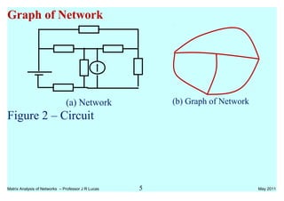
The document discusses matrix analysis of networks, focusing on understanding the structure and properties of interconnected systems. It explains fundamental concepts such as tree and co-tree formations, the use of Kirchhoff's laws in matrix form, and techniques for circuit analysis using mesh and nodal methods. The analysis includes equations, graphs, and examples to illustrate how to apply matrix techniques for solving circuit problems.


![a1k .i1 + a2k . i2 + a3k .i3 + a4k .i4 + ...... ....... ..... a7k .i7 = 0
or ∑
=
=⋅
b
j
jjk ia
1
0
at kth
node, for all k
Collection of equations, for each node k, would give
[ ] )1()1()(
0
×××
=⋅
nb
b
bn
It
A
In [A]t
, row vectors are dependant, since sum is zero.
[A]t
written with one row less, giving only (n-1) rows.
[A]t
– node-branch incidence matrix, (n-1)×b.
[A] – branch-node incidence matrix, b× (n-1)
ajk = +1 if jth
current is directed away from the kth
node
ajk = −1 if jth
current is directed towards the kth
node
Matrix Analysis of Networks – Professor J R Lucas 16 May 2011](https://image.slidesharecdn.com/240164036-ee2092-4-2011-matrix-analysis-150913071309-lva1-app6891/85/240164036-ee2092-4-2011-matrix-analysis-16-320.jpg)
![ajk = 0 if jth
current is not incident on the kth
node
Kirchoff’s voltage Law in matrix form
∑
=
=⋅
b
r
rrs vb
1
0
for sth
loop, for all s;
where brs = −1, 0, or +1
[ ] )1()1()(
0
×××
=⋅
lb
b
bl
Vt
B
[B]t
– mesh-branch incidence matrix, (l×b)
[B] – branch-mesh incidence matrix, (b×l)
brs = +1if rth
current is in same direction as sth
loop
brs = −1if rth
current is in opposite direction to sth
loop
brs = 0 if rth
current is in the not part of the sth
loop
Ohm’s Law in matrix form
Matrix Analysis of Networks – Professor J R Lucas 17 May 2011
0
0
0+1
-1
-1
0
-1
+1
s
0
0
0](https://image.slidesharecdn.com/240164036-ee2092-4-2011-matrix-analysis-150913071309-lva1-app6891/85/240164036-ee2092-4-2011-matrix-analysis-17-320.jpg)

![With a voltage source only
vk = – egk + Zk ik
for all branches k = 1, 2, ....... b
and in matrix form as[ ] bbgbb IZEV +−=
With a current source only
ik = Yk vk – igk
for all branches k = 1, 2, .... ... b
and in matrix form as
[ ] bbgbb VYII +−=
, where [Yb] = [Zb]-1
Matrix Analysis of Networks – Professor J R Lucas 19 May 2011
egk
Zk
vk
ik
igk
Ykik
vk](https://image.slidesharecdn.com/240164036-ee2092-4-2011-matrix-analysis-150913071309-lva1-app6891/85/240164036-ee2092-4-2011-matrix-analysis-19-320.jpg)
![In Summary
From Kirchoff’s Laws
[ ] )1()1()(
0
×××
=⋅
nb
b
bn
It
A
(1) (n-1) independent equations
[ ] )1()1()(
0
×××
=⋅
lb
b
bl
Vt
B
(2) l independent equations
and from Ohm’s Law
[ ] bbgbb IZEV +−=
(3) b independent equations
or [ ] bbgbb VYII +−=
(3)* b independent equations
Thus total number of independent equations is
n – 1 + l + b = b + b = 2 b
2b independent equations
2b unknowns (b branch currents and b branch voltages)
Matrix Analysis of Networks – Professor J R Lucas 20 May 2011](https://image.slidesharecdn.com/240164036-ee2092-4-2011-matrix-analysis-150913071309-lva1-app6891/85/240164036-ee2092-4-2011-matrix-analysis-20-320.jpg)

![Mesh Analysis
− Eliminate the branch voltages from the equations.
− Reduce remaining currents to a minimum using
Kirchoff’s current law.
Apply Kirchoff’s voltage law for solution.
Define a set of mesh currents, mI
.
Branch currents bI
related to mesh currents mI
by an
algebraic summation.
[ ] mb IBI =
(4)
Eliminate Vb from the equations,
Pre-multiply equation (3) by [B]t
.
Matrix Analysis of Networks – Professor J R Lucas 22 May 2011](https://image.slidesharecdn.com/240164036-ee2092-4-2011-matrix-analysis-150913071309-lva1-app6891/85/240164036-ee2092-4-2011-matrix-analysis-22-320.jpg)
![[ ] [ ] [ ] [ ] bb
t
gb
t
b
t
IZBEBVB +−=
from equation (2), [B]t
Vb = 0.
Also [ ] mb IBI =
∴ [ ] [ ] [ ][ ] mb
t
gb
t
IBZBEB =
[B]t
Vb = 0 → sum of voltages around a loop is zero.
i.e. [B]t
Vb → sum of voltages around a loop.
∴ [B]t
Egb → sum of source voltages around a loop.
Defined as mesh source voltage vector Egm .
i.e. Egm = [B]t
Egb
∴ Egm = [ ] [ ][ ] [ ] mmmb
t
IZIBZB =
Matrix Analysis of Networks – Professor J R Lucas 23 May 2011](https://image.slidesharecdn.com/240164036-ee2092-4-2011-matrix-analysis-150913071309-lva1-app6891/85/240164036-ee2092-4-2011-matrix-analysis-23-320.jpg)
![where [Zm] = [ ] [ ][ ]BZB b
t
corresponds to l equations
[B] also known as the tie-set matrix
(as its elements tie the loop together)
Unknowns are l values of current Im
Original 2b equations and 2b unknowns reduced to
l equations and l unknowns.
Elements of [Zm] can be obtained either from above
mathematics, or by inspection as follows.
Simple evaluation of [Zm] and Egm
zjj = self impedance of mesh j
= sum of all branch impedances in mesh j
Matrix Analysis of Networks – Professor J R Lucas 24 May 2011](https://image.slidesharecdn.com/240164036-ee2092-4-2011-matrix-analysis-150913071309-lva1-app6891/85/240164036-ee2092-4-2011-matrix-analysis-24-320.jpg)


![This gives the Branch-Mesh incidence matrix [B].
Mesh–Branch incidence matrix [B]t
can also
independently by writing the relation between the
mesh direction and the branch direction.
[ ]
−−
−=
110010
011100
000101
t
B
Notice that this corresponds to the transpose of the
earlier written matrix.
Matrix Analysis of Networks – Professor J R Lucas 28 May 2011](https://image.slidesharecdn.com/240164036-ee2092-4-2011-matrix-analysis-150913071309-lva1-app6891/85/240164036-ee2092-4-2011-matrix-analysis-28-320.jpg)
![Vector of branch source voltages is
Branch impedance matrix is
[ ]
−
=
600000
0100000
0020000
00012000
0000100
0000020
j
j
j
Zb
Egm = [B]t
Egb , and [Zm] = [B]t
[Zb] [B]
∠
∠
−−
−=
0
0
0
0
87.36100
0100
110010
011100
000101
0
0
gmE
, Egm =
∠−
∠
0
0
87.36100
0
0100
Matrix Analysis of Networks – Professor J R Lucas 29 May 2011
∠
∠
=
0
0
0
0
87.36100
0100
0
0
gbE](https://image.slidesharecdn.com/240164036-ee2092-4-2011-matrix-analysis-150913071309-lva1-app6891/85/240164036-ee2092-4-2011-matrix-analysis-29-320.jpg)
![[ ]
−
−
−
−
−−
−=
100
110
010
011
100
001
600000
0100000
0020000
00012000
0000100
0000020
110010
011100
000101
j
j
j
Zm
[ ]
−
−
−
−−
−=
600
10100
0200
0120120
1000
0020
110010
011100
000101
j
jj
j
Zm
=
+−
−−
−
620100
1012030120
0120100
j
jj
jj
Both Egm and Zm could have been written by inspection.
Thus
∠−
∠
0
0
87.36100
0
0100
=
+−
−−
−
3
2
1
620100
1012030120
0120100
I
I
I
j
jj
jj
Equations may be solved by inversion or otherwise.
Matrix Analysis of Networks – Professor J R Lucas 30 May 2011](https://image.slidesharecdn.com/240164036-ee2092-4-2011-matrix-analysis-150913071309-lva1-app6891/85/240164036-ee2092-4-2011-matrix-analysis-30-320.jpg)
![
∠−
∠
−−−×−×−
×−+−+−
×−+−−+−
∆
=
0
0
2
2
3
2
1
87.36100
0
0100
)120()12030(1001010010120
10100)620(100)620(120
10120)620(12010)620)(12030(
1
jjjjj
jjjjj
jjjjj
I
I
I
−−
+−−−−
−+−+−
−+−−
∆
=
6080
0
100
1440012000300010001200
100060020007202400
1200720240022201220
1
3
2
1
jjjj
jjj
jjjj
I
I
I
∆ = (1220 – j2220)×(–j100) + (720 –
j2400) ×(j120) + (–j1200) ×0
= – j122000 – 222000 + j 86400 + 288000
= 66000 – j 35600 = 74989∠-28.34o
I1 = (122000 – j 222000 + 0 + j 96000 – 72000)/74989∠-28.34o
= (50000 – j 126000)/ 74989∠-28.34o
= 135558∠-68.36o
/74989∠-28.34o
= 1.808∠-40.02o
A
[Note: Inversion has not been checked so answers may be in error.]
Currents I2 and I3 can be similarly determined.
The branch currents i1, i2, ..... may then be determined from the matrix equation.
[Normally branch 6 would have been marked as part of branch 2]
Matrix Analysis of Networks – Professor J R Lucas 31 May 2011](https://image.slidesharecdn.com/240164036-ee2092-4-2011-matrix-analysis-150913071309-lva1-app6891/85/240164036-ee2092-4-2011-matrix-analysis-31-320.jpg)
![Nodal Analysis
− eliminate branch currents from the equations.
− Reduce number of remaining voltages to a minimum
using Kirchoff’s voltage law.
Apply Kirchoff’s current law for solution.
Define a set of nodal voltages, NV
which are node pair
voltages (i.e. voltage across a pair of nodes)
Branch voltages bV
are related to nodal voltages NV
by an
algebraic summation.
[ ] Nb VAV =
(5)
[A] too does not have the reference node.
Matrix Analysis of Networks – Professor J R Lucas 32 May 2011](https://image.slidesharecdn.com/240164036-ee2092-4-2011-matrix-analysis-150913071309-lva1-app6891/85/240164036-ee2092-4-2011-matrix-analysis-32-320.jpg)
![Pre-multiply equation (3)* by [A]t
.
[ ] [ ] [ ] [ ] bb
t
gb
t
b
t
VYAIAIA +−=
from equation (1), [A]t
Ib = 0 .
Substituting from (5)
[ ] [ ] [ ][ ] Nb
t
gb
t
VAYAIA +−=0
[ ] [ ] [ ][ ] Nb
t
gb
t
VAYAIA =
IgN = [YN]VN
where [ ] gb
t
gN IAI =
, and
[ ] [ ] [ ][ ]AYAY b
t
N =
Source nodal current vector IgN and the nodal
admittance matrix [YN] could be written by inspection.
yii = sum of all branch admittances incident at node i
Matrix Analysis of Networks – Professor J R Lucas 33 May 2011](https://image.slidesharecdn.com/240164036-ee2092-4-2011-matrix-analysis-150913071309-lva1-app6891/85/240164036-ee2092-4-2011-matrix-analysis-33-320.jpg)

![IgN = [YN]VN
is first solved to give VN and the branch voltages
and branch currents then obtained using the matrix equations.
Matrix Analysis of Networks – Professor J R Lucas 35 May 2011](https://image.slidesharecdn.com/240164036-ee2092-4-2011-matrix-analysis-150913071309-lva1-app6891/85/240164036-ee2092-4-2011-matrix-analysis-35-320.jpg)
![Example 2
Example 1 has been reformulated as a problem with
current sources rather than with voltage sources.
[If voltage sources are present, they would first have to
be converted to current sources].
Matrix Analysis of Networks – Professor J R Lucas 36 May 2011
5∠-900
A
j20 Ω
j6 Ω
-j120 Ω
8.575∠5.910
A10 Ω
20 Ω
10 Ω
i1
i4
i3
i5
i2
V1
V2](https://image.slidesharecdn.com/240164036-ee2092-4-2011-matrix-analysis-150913071309-lva1-app6891/85/240164036-ee2092-4-2011-matrix-analysis-36-320.jpg)
![Network may also be drawn in terms of admittances.
The branch-node incidence matrix [A],
branch injected current Igb, and
branch admittance matrix may be written,
with reference selected as earthed node as follows.
Matrix Analysis of Networks – Professor J R Lucas 37 May 2011
∠
∠
i1
i4
i3
i5
i2
V1
V2](https://image.slidesharecdn.com/240164036-ee2092-4-2011-matrix-analysis-150913071309-lva1-app6891/85/240164036-ee2092-4-2011-matrix-analysis-37-320.jpg)
![[ ]
−
−
−
=
10
11
01
10
01
A
, Igb =
∠
−∠
0
0
0
91.5575.8
905
o
o
,
[ ]
−
−
=
1.00000
005.0000
00008333.000
0000441.00735.00
000005.0
j
j
j
Yb
As in mesh analysis, nodal current injection vector and nodal
admittance matrix may be written from first principles.
Left as an exercise for you to work out.
This is worked by inspection.
[ ] [ ]
−++−
−++−
=
∠
−∠
=
0441.00735.01.005.005.0
05.005.000833.005.0
,
91.5575.8
905
j
jj
YI No
o
gN
−++−
−++−
=
∠
−∠
∴
2
1
0441.00735.01.005.005.0
05.005.000833.005.0
91.5575.8
905
V
V
j
jj
o
o
∠
−∠
++−
−++
∆
=
∴ o
o
jj
j
V
V
91.5575.8
905
05.000833.005.005.0
05.00441.00735.01.005.01
2
1
∆ = (–j0.05+j0.00833+0.05)(0.05+0.1+0.0735–j0.0441) – 0.052
Matrix Analysis of Networks – Professor J R Lucas 38 May 2011](https://image.slidesharecdn.com/240164036-ee2092-4-2011-matrix-analysis-150913071309-lva1-app6891/85/240164036-ee2092-4-2011-matrix-analysis-38-320.jpg)


![Definitions
Driving point impedance is defined as ratio of applied
voltage (driving point voltage) across a node-pair to
the current entering at the same port.
[input impedance of network seen from particular port]
Driving point impedance at Port 1 = V1/I1
Driving point impedance at Port 2 = V2/I2
Driving point admittance is similarly defined as the
ratio of the current entering at a port to the applied
voltage across the same node-pair.
Driving point admittance at Port 1 = I1/V1
Driving point admittance at Port 2 = I2/V2
Matrix Analysis of Networks – Professor J R Lucas 46 May 2011
](https://image.slidesharecdn.com/240164036-ee2092-4-2011-matrix-analysis-150913071309-lva1-app6891/85/240164036-ee2092-4-2011-matrix-analysis-46-320.jpg)


![Example 3
Find impedance parameters of the two port T – network.
With port 2 on open circuit
ba ZZ
II
V
z +=
=
=
021
1
11
bZ
II
V
z =
=
=
021
2
21
similarly with port 1 open,
z12 = Zb
z22 = Zb + Zc
(b) Admittance Parameters (y-parameters)
or Short-circuit parameters
Matrix Analysis of Networks – Professor J R Lucas 52 May 2011
[ ]
+
+
=→
cbb
bba
ZZZ
ZZZ
Z](https://image.slidesharecdn.com/240164036-ee2092-4-2011-matrix-analysis-150913071309-lva1-app6891/85/240164036-ee2092-4-2011-matrix-analysis-52-320.jpg)

![Example 4
Find admittance parameters of the 2 port π–network.
y11 = 021
1
=VV
I
= Ya + Yb
y21 = 021
2
=VV
I
= – Yb
Matrix Analysis of Networks – Professor J R Lucas 54 May 2011
→[Y] =
+−
−+
cbb
bba
YYY
YYY](https://image.slidesharecdn.com/240164036-ee2092-4-2011-matrix-analysis-150913071309-lva1-app6891/85/240164036-ee2092-4-2011-matrix-analysis-54-320.jpg)

![Example 5
Find ABCD parameters.
A = c
cb
Y
YY +
, B = cY
1
C = c
accbba
Y
YYYYYY ++
and D =
c
ca
Y
YY +
[For symmetrical
network, Ya = Yb , A = D].
A.D – B.C = c
accbba
cc
ca
c
cb
Y
YYYYYY
YY
YY
Y
YY ++
⋅−
+
⋅
+ 1
= 2
2
)(
c
accbbaccbacab
Y
YYYYYYYYYYYYY ++−+++
=1
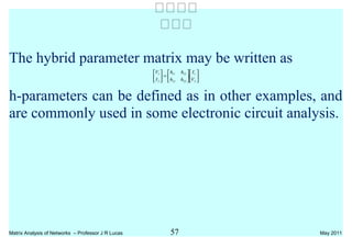
(d) Hybrid Parameters (h-parameters)
Matrix Analysis of Networks – Professor J R Lucas 56 May 2011
](https://image.slidesharecdn.com/240164036-ee2092-4-2011-matrix-analysis-150913071309-lva1-app6891/85/240164036-ee2092-4-2011-matrix-analysis-56-320.jpg)

![[Z] = [Zr] + [Zs]
Matrix Analysis of Networks – Professor J R Lucas 59 May 2011](https://image.slidesharecdn.com/240164036-ee2092-4-2011-matrix-analysis-150913071309-lva1-app6891/85/240164036-ee2092-4-2011-matrix-analysis-59-320.jpg)

![at port 2, Ir2 + Is2 = I2, and Vr2 = Vs2 = V2
[Y] = [Yr] + [Ys]
(c) Cascade connection of networks
Output of one network becomes input to next.
Ir2 = Is1
Vr2 = Vs1
=
2
2
1
1
r
r
rr
rr
r
r
I
V
DC
BA
I
V
,
=
2
2
1
1
s
s
ss
ss
s
s
I
V
DC
BA
I
V
=
2
2
1
1
I
V
DC
BA
DC
BA
I
V
ss
ss
rr
rr
ABCD matrix of component networks
Matrix Analysis of Networks – Professor J R Lucas 61 May 2011
](https://image.slidesharecdn.com/240164036-ee2092-4-2011-matrix-analysis-150913071309-lva1-app6891/85/240164036-ee2092-4-2011-matrix-analysis-61-320.jpg)