The document presents unit 4 notes on artificial intelligence, emphasizing classical planning, algorithms, and state-space search methodologies necessary for B.Tech students in AI and ML. It covers classical planning definitions, applications, and various algorithms including forward and backward state-space planning, as well as planning graphs. Key problems such as air cargo transport and the spare tire problem are discussed, along with the benefits and drawbacks of classical planning approaches.

1. 22PCOAM11
INTRODUCTION TO ARTIFICAL
INTELLIGENCE
UNIT 4 NOTES
B.TECH
II YEAR – IV SEM (R22)
(2024-2025)
Prepared
By
Asst.Prof.M.Gokilavani
Department of Artificial Intelligence and Machine Learning

2. R22 B.Tech. CSE (AI and ML) Syllabus JNTU Hyderabad
INTRODUCTION TO ARTIFICIAL INTELLIGENCE
B.Tech. II Year II Sem. L T P C
3 0 0 3
Prerequisite: Knowledge on Data Structures.
Course Objectives:
● To learn the distinction between optimal reasoning Vs. human like reasoning.
● To understand the concepts of state space representation, exhaustive search, heuristic
● search together with the time and space complexities.
● To learn different knowledge representation techniques.
● To understand the applications of AI, namely game playing, theorem proving, and machine
learning.
Course Outcomes:
● Learn the distinction between optimal reasoning Vs human like reasoning and formulate an
efficient problem space for a problem expressed in natural language. Also select a search
algorithm for a problem and estimate its time and space complexities.
● Apply AI techniques to solve problems of game playing, theorem proving, and machine
learning.
● Learn different knowledge representation techniques.
● Understand the concepts of state space representation, exhaustive search, heuristic search
together with the time and space complexities.
● Comprehend the applications of Probabilistic Reasoning and Bayesian Networks.
● Analyze Supervised Learning Vs. Learning Decision Trees
UNIT - I
Introduction to AI - Intelligent Agents, Problem-Solving Agents,
Searching for Solutions - Breadth-first search, Depth-first search, Hill-climbing search, Simulated
annealing search, Local Search in Continuous Spaces.
UNIT-II
Games - Optimal Decisions in Games, Alpha–Beta Pruning, Defining Constraint Satisfaction Problems,
Constraint Propagation, Backtracking Search for CSPs, Knowledge-Based Agents, Logic-
Propositional Logic, Propositional Theorem Proving: Inference and proofs, Proof by resolution, Horn
clauses and definite clauses.
UNIT-III
First-Order Logic - Syntax and Semantics of First-Order Logic, Using First Order Logic, Knowledge
Engineering in First-Order Logic. Inference in First-Order Logic: Propositional vs. First-Order Inference,
Unification, Forward Chaining, Backward Chaining, Resolution.
Knowledge Representation: Ontological Engineering, Categories and Objects, Events.
UNIT-IV
Planning - Definition of Classical Planning, Algorithms for Planning with State Space Search, Planning
Graphs, other Classical Planning Approaches, Analysis of Planning approaches. Hierarchical Planning.
UNIT-V
Probabilistic Reasoning:
Acting under Uncertainty, Basic Probability Notation Bayes’ Rule and Its Use, Probabilistic Reasoning,
Representing Knowledge in an Uncertain Domain, The Semantics of Bayesian Networks, Efficient

3. R22 B.Tech. CSE (AI and ML) Syllabus JNTU Hyderabad
Representation of Conditional Distributions, Approximate Inference in Bayesian Networks, Relational
and First- Order Probability.
TEXT BOOK:
1. Artificial Intelligence: A Modern Approach, Third Edition, Stuart Russell and Peter Norvig,
Pearson Education.
REFERENCE BOOKS:
1. Artificial Intelligence, 3rd Edn., E. Rich and K. Knight (TMH)
2. Artificial Intelligence, 3rd Edn., Patrick Henny Winston, Pearson Education.
3. Artificial Intelligence, Shivani Goel, Pearson Education.
4. Artificial Intelligence and Expert systems – Patterson, Pearson Education.

4. UNIT IV
Planning
Classical Planning: Definition of Classical Planning, Algorithms for Planning with State-Space Search,
Planning Graphs, other Classical Planning Approaches, Analysis of Planning Approaches, Hierarchical
Planning.
CLASSICAL PLANNING:
1. DEFINITION OF CLASSICAL PLANNING:
Classical Planning is the planning where an agent takes advantage of the problem structure to construct
complex plans of an action. The agent performs three tasks in classical planning:
 Planning: The agent plans after knowing what the problem is.
 Acting: It decides what action it must take.
 Learning: The actions taken by the agent make him learn new things.
A language known as PDDL (Planning Domain Definition Language) is used to represent all actions
into one action schema.
PDLL describes the four basic things needed in a search problem:
 Initial state: It is the representation of each state as the conjunction of the ground and
functionless atoms.
 Actions: It is defined by a set of action schemas that implicitly define the ACTION
() and RESULT () functions.
 Result: It is obtained by the set of actions used by the agent.
 Goal: It is the same as a precondition, which is a conjunction of literals (whose value is either
positive or negative).
There are various examples that will make PDLL understandable:
 Air cargo transport
 The spare tire problem

5.  The blocks world and many more.
i. Air cargo transport:
This problem can be illustrated with the help of the following actions:
 Load: This action is taken to load cargo.
 Unload: This action is taken to unload the cargo when it reaches its destination.
 Fly: This action is taken to fly from one place to another.
Therefore, the Air cargo transport problem is based on loading and unloading the cargo and flying it
from one place to another.
Below is the PDLL description for Air cargo transport:
Init (On(C1, SFO) ? On(C2, JFK) ? On(P1, SFO) ? On(P2, JFK)?
Cargo(C1) ? Cargo(C2) ? Plane(P1) ? Plane(P2)
? Airport (JFK) ? Airport (SFO))
Goal (On(C1, JFK) ? On(C2, SFO))
Action(Load (c, p, a),
PRECOND: On(c, a) ? On(p, a) ? Cargo(c) ? Plane(p) ? Airport (a)
EFFECT: ? On(c, a) ? In(c, p))
Action(Unload(c, p, a),
PRECOND: In(c, p) ? On(p, a) ? Cargo(c) ? Plane(p) ? Airport (a)
EFFECT: On(c, a) ? ?In(c, p))
Action(Fly(p, from, to),
PRECOND: On(p, from) ? Plane(p) ? Airport (from) ? Airport (to)
EFFECT: ? On(p, from) ? On(p, to))
The above-described actions, (i.e., load, unload, and fly) affects the following two predicates:
 (c,p): In this, the cargo is inside the plane p.
 (x,a): In this, the object x is at the airport a. Here, object can be the cargo or plane.
It is to be noted that when the plan flies from one place to another, it should carry all cargo inside it. It
becomes difficult with the PDLL to give solution for such a problem. Because PDLL do not have the
universal quantifier. Thus, the following approach is used:

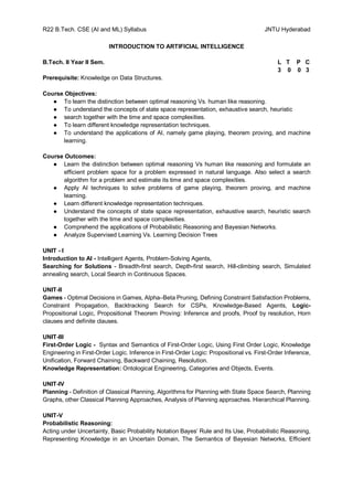
6.  piece of cargo ceases to be on anywhere when it is in a plane.
 the cargo only becomes on the new airport when it is unloaded.
Therefore, the planning for the solution is:
Load (C1, P1, SFO), Fly (P1, SFO, JFK), Unload (C1, P1, JFK),
Load (C2, P2, JFK), Fly (P2, JFK, SFO), Unload (C2, P2, SFO)]
Note: Some problems can be ignored because they does not cause any problem in planning.
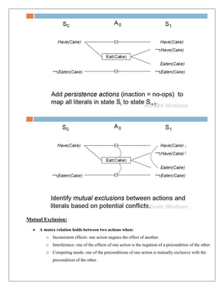
ii. The spare tire problem:
The problem is that the agent needs to change the flat tire. The aim is to place a good spare tire over the
car’s axle. There are four actions used to define the spare tire problem:
1. Remove the spare from the trunk.
2. Remove the flat spare from the axle.
3. Putting the spare on the axle.
4. Leave the car unattended overnight. Assuming that the car is parked at an unsafe neighbourhood.
The PDLL description for the spare tire problem is:
Init(Tire1(Flat ) ? Tire1(Spare) ? At(Flat , Axle) ? At(Spare, Trunk
))
Goal (At(Spare, Axle))
Action(Remove(obj , loc),
PRECOND: At(obj , loc)
EFFECT: ? At(obj , loc) ? At(obj , Ground))
Action(PutOn(t , Axle),
PRECOND: Tire1(t) ? At(t , Ground) ?¬At(Flat , Axle)
EFFECT: ? At(t , Ground) ? At(t , Axle))
Action(LeaveOvernight ,
PRECOND:
EFFECT: ? At(Spare, Ground) ?¬At(Spare, Axle) ?¬At(Spare, Trunk)
?¬At(Flat, Ground) ?¬At(Flat , Axle) ?¬At(Flat, Trunk))

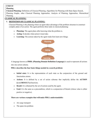
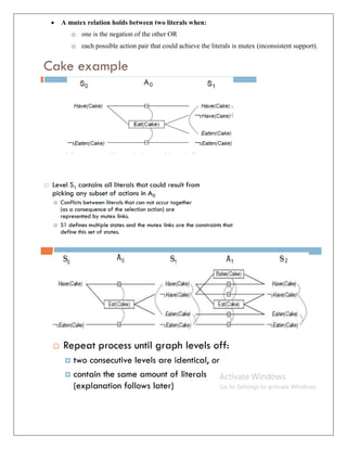
7. The solution to the problem is:
[Remove(Flat,Axle),Remove(Spare,Trunk), PutOn(Spare, Axle)].
iii. Block-world planning problem
 The block-world problem is known as the Sussman anomaly.
 The non-interlaced planners of the early 1970s were unable to solve this problem. Therefore,
it is considered odd.
 When two sub-goals, G1 and G2, are given, a non-interleaved planner either produces a plan
for G1 that is combined with a plan for G2 or vice versa.
 In the block-world problem, three blocks labelled 'A', 'B', and 'C' are allowed to rest on a flat
surface. The given condition is that only one block can be moved at a time to achieve the
target.
The start position and target position are shown in the following diagram.
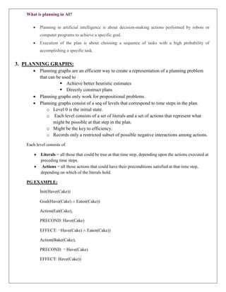
Components of the planning system
The plan includes the following important steps:
o Choose the best rule to apply the next rule based on the best available guess.
o Apply the chosen rule to calculate the new problem condition.
o Find out when a solution has been found.
o Detect dead ends so they can be discarded and direct system effort in more useful directions.
o Find out when a near-perfect solution is found.

8. Target stack plan
o It is one of the most important planning algorithms used by STRIPS.
o Stacks are used in algorithms to capture the action and complete the target. A knowledge base is
used to hold the current situation and actions.
o A target stack is like a node in a search tree, where branches are created with a choice of action.
The important steps of the algorithm are mentioned below:
1. Start by pushing the original target onto the stack. Repeat this until the pile is empty. If the stack
top is a mixed target, push its unsatisfied sub-targets onto the stack.
2. If the stack top is a single unsatisfied target, replace it with action and push the action
precondition to the stack to satisfy the condition.
iii. If the stack top is an action, pop it off the stack, execute it and replace the knowledge base with the
action's effect.
If the stack top is a satisfactory target, pop it off the stack.
The complexity of the classical planning:
In classical planning, there occur following two decision problems:
1. Plan SAT: It is the question asking if there exists any plan that solves a planning problem.
2. Bounded Plan SAT: It is the question asking if there is a solution of length k or less than it.
We found that:
 Plan SAT and Bounded Plan SAT are decidable for classical planning.
 Both decision problems lie in the complexity class PSPACE, which is larger than NP.
Note: PSPACE is the class which refers to those problems that can be solved via deterministic Turing
machine under a polynomial time space.
From the above, it can be concluded that:
1. Plan SAT is P whereas Bounded Plan SAT is NP-complete.
2. Optimal planning is hard with respect to sub-optimal planning.
Advantages of Classical Planning
There are the following advantages of Classical planning:

9.  It has provided the facility to develop accurate domain-independent heuristics.
 The systems are easy to understand and work efficiently.
2. ALGORITHMS FOR PLANNING WITH STATE-SPACE SEARCH:
What is a Plan?
We require domain description, task specification, and goal description for any planning system. A plan
is considered a sequence of actions, and each action has its preconditions that must be satisfied before
it can act and some effects that can be positive or negative.
So, we have Forward State Space Planning (FSSP) and Backward State Space Planning (BSSP) at
the basic level.
1. Forward State Space Planning (FSSP)
 Works like regular search: start with the initial state, expand the graph by computing successors.

10.  The successors are computed by using the applicable actions and finding the resulting states
 FSSP behaves in the same way as forwarding state-space search. It says that given an initial state
S in any domain, we perform some necessary actions and obtain a new state S' (which also
contains some new terms), called a progression.
 It continues until we reach the target position. Action should be taken in this matter.
Properties of forward state space planning:
 There will be a lot of irrelevant actions, i.e., actions that will not contribute to the final plan
 The state space is large.
o Disadvantage: Large branching factor
o Advantage: The algorithm is Sound
2. Backward State Space Planning (BSSP)
BSSP behaves similarly to backward state-space search. In this, we move from the target state g to the
sub-goal g, tracing the previous action to achieve that goal. This process is called regression (going back
to the previous goal or sub-goal). These sub-goals should also be checked for consistency. The action
should be relevant in this case.
Properties of backward state space planning:
 Irrelevant actions will be less of an issue because we are starting with the goal.
 The branching factor is low, but regression gives a set of states rather than a single state.
 Thus, it is hard to develop heuristics (the situation is like partial order planners).
o Disadvantages: not sound algorithm (sometimes inconsistency can be found)
o Advantage: Small branching factor (much smaller than FSSP)
So for an efficient planning system, we need to combine the features of FSSP and BSSP, which gives
rise to target stack planning which will be discussed in the next article.

11. What is planning in AI?
 Planning in artificial intelligence is about decision-making actions performed by robots or
computer programs to achieve a specific goal.
 Execution of the plan is about choosing a sequence of tasks with a high probability of
accomplishing a specific task.
3. PLANNING GRAPHS:
 Planning graphs are an efficient way to create a representation of a planning problem
that can be used to
 Achieve better heuristic estimates
 Directly construct plans
 Planning graphs only work for propositional problems.
 Planning graphs consist of a seq of levels that correspond to time steps in the plan.
o Level 0 is the initial state.
o Each level consists of a set of literals and a set of actions that represent what
might be possible at that step in the plan.
o Might be the key to efficiency.
o Records only a restricted subset of possible negative interactions among actions.
Each level consists of
 Literals = all those that could be true at that time step, depending upon the actions executed at
preceding time steps.
 Actions = all those actions that could have their preconditions satisfied at that time step,
depending on which of the literals hold.
PG EXAMPLE:
Init(Have(Cake))
Goal(Have(Cake)  Eaten(Cake))
Action(Eat(Cake),
PRECOND: Have(Cake)
EFFECT: ¬Have(Cake)  Eaten(Cake))
Action(Bake(Cake),
PRECOND: ¬ Have(Cake)
EFFECT: Have(Cake))

13. Mutual Exclusion:
 A mutex relation holds between two actions when:
o Inconsistent effects: one action negates the effect of another.
o Interference: one of the effects of one action is the negation of a precondition of the other.
o Competing needs: one of the preconditions of one action is mutually exclusive with the
precondition of the other.

14.  A mutex relation holds between two literals when:
o one is the negation of the other OR
o each possible action pair that could achieve the literals is mutex (inconsistent support).

15. The GRAPHPLAN Algorithm:
Extract a solution directly from the PG
Example:

16. EXPAND-GRAPH also looks for mutex relations
 Inconsistent effects
o E.g. Remove(Spare, Trunk) and LeaveOverNight due to At(Spare,Ground) and not
At(Spare, Ground)
 Interference
o E.g. Remove(Flat, Axle) and LeaveOverNight At(Flat, Axle) as PRECOND and not
At(Flat,Axle) as EFFECT
 Competing needs
o E.g. PutOn(Spare,Axle) and Remove(Flat, Axle) due to At(Flat.Axle) and not At(Flat,
Axle)
 Inconsistent support
o E.g. in S2, At(Spare,Axle) and At(Flat,Axle)

17. GRAPHPLAN Termination:
 Termination? YES
 PG are monotonically increasing or decreasing:
o Literals increase monotonically
o Actions increase monotonically
o Mutexes decrease monotonically
 Because of these properties and because there is a finite number of actions and literals, every
PG will eventually level off.
4. OTHER CLASSICAL PLANNING APPROACHES:
The most popular and effective approaches to fully automated planning are:
• Translating to a Boolean satisfiability (SAT) problem
• Forward state-space search with carefully crafted heuristics
• Search using a planning graph
(REFER Your PPT for Notes)
5. Hierarchical Planning (Refer PPT for notes)