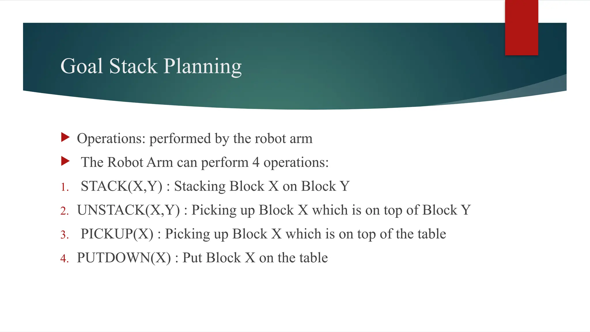
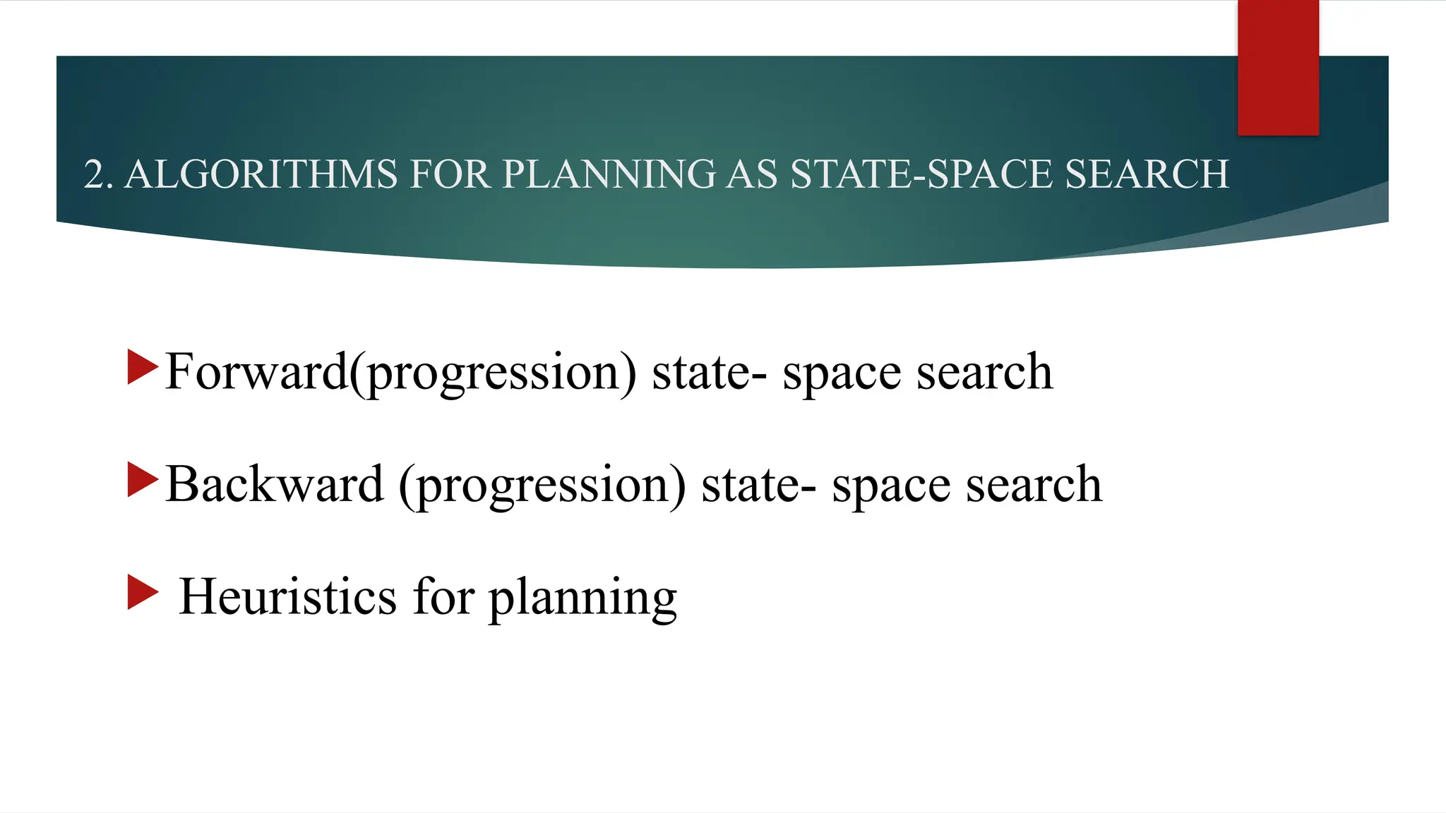
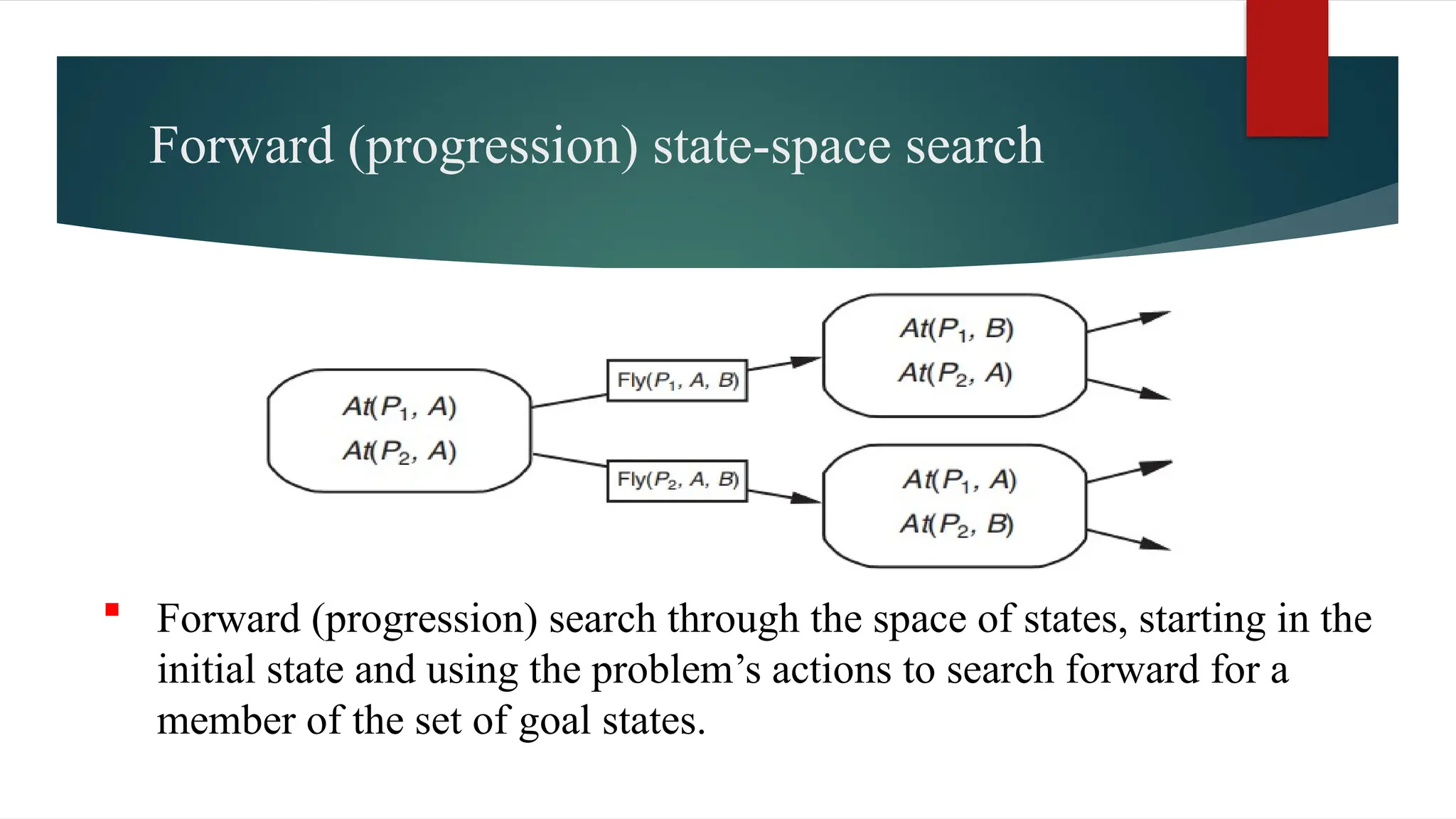
The document covers classical planning in artificial intelligence, emphasizing the importance of decision-making actions to achieve specific goals. It introduces various concepts, such as the blocks world problem and goal stack planning, as well as algorithms for planning that can be approached through state-space search methods. Additionally, it discusses heuristics for efficient planning, the use of planning graphs, and the Graphplan algorithm for determining goal reachability and mutual achievability.

1. Classical planning

2. 1
.
What is the planning
 A plan: is considered a sequence of actions, and each action has its
preconditions that must be satisfied before it can act and some
effects that can be positive or negative.

3. What is the Role of Planning in Artificial
Intelligence
 Planning is an important part of Artificial Intelligence which deals with
the tasks and domains of a particular problem. Planning is considered
the logical side of acting.
 Everything we humans do is with a definite goal in mind, and all our
actions are oriented towards achieving our goal. Similarly, Planning is
also done for Artificial Intelligence.

4. What is the Role of Planning in Artificial
Intelligence
 For example, Planning is required to reach a particular destination.
It is necessary to find the best route in Planning, but the tasks to be
done at a particular time and why they are done are also very
important.
 That is why Planning is considered the logical side of acting. In
other words, Planning is about deciding the tasks to be performed
by the AI system and the system's functioning under domain
independent conditions.

5. Planning in AI
 Planning in AI is about decision-making actions
performed by agents (robots or computer programs) to
achieve a specific goal.
 Execution of the plan is about choosing a sequence of
tasks with a high probability of accomplishing a specific
task

6. Example: The blocks world problem
 One of the most famous planning domains is known as the blocks
world.
 This domain consists of a set of cube-shaped blocks sitting on a
table.2 The blocks can be stacked, but only one block can fit directly
on top of another.
 A robot arm can pick up a block and move it to another position,
either on the table or on top of another block.
 The arm can pick up only one block at a time, so it cannot pick up a
block that has another one on it. The goal will always be to build
one or more stacks of blocks, specified in terms of what blocks are
on top of what other blocks.

7. Example: The blocks world problem
 In the block-world problem, three blocks labeled 'A', 'B',
and 'C' are allowed to rest on a flat surface.
 The given condition is that only one block can be moved
at a time to achieve the target.

8. Example: The blocks world problem
There are ‘N’ number of Blocks resting on a table with a
specified sequence.
• Goal: arrange in a desired sequence.
• Available moves:
1) Put a Block on the table.
2) Put a Block on top of another one.
• State is represented using a sequence of blocks in
current position

9. Example: The blocks world problem
 The blocks world has two kinds of components:
• A table top with three places p, q, and r.
• A variable number of blocks A, B, C, D., that can be arranged in places
on the table or stacked on one another
 A legal move is to transfer a block from one place or block onto another
place or block, with these restrictions:
• The moved block must not have another block on top of it.
• No other blocks are moved in the process.

10. What is Goal Stack Planning
?
 Goal Stack Planning is one of the earliest methods in artificial
intelligence in which we work backwards from the goal state to the
initial state.
 We start at the goal state and we try fulfilling the preconditions
required to achieve the initial state. These preconditions in turn
have their own set of preconditions, which are required to be
satisfied first. We keep solving these “goals” and “sub-goals” until
we finally arrive at the Initial State. We make use of a stack to hold
these goals that need to be fulfilled as well the actions that we need
to perform for the same.

11. What is Goal Stack Planning
?
 Representing the configurations as a list of “predicates”
 Predicates can be thought of as a statement which helps us convey the
information about a configuration in Blocks World.
• Given below are the list of predicates as well as their intended meaning
1. ON(B,A): Block B is on A.
2. ONTABLE(A): A is on table.
3. CLEAR(B): Nothing is on top of B.
4. HOLDING(C): Arm is holding C.
5. ARMEMPTY: Arm is holding nothing.

12. Goal Stack Planning
 Initial State :
ON(B,A) ONTABLE(A) ONTABLE(C) ONTABLE(D)
∧ ∧ ∧ ∧
CLEAR(B) CLEAR(C) CLEAR(D) ARMEMPTY
∧ ∧ ∧
 Goal State :
ON(C,A) ON(B,D) ONTABLE(A) ONTABLE(D)
∧ ∧ ∧ ∧
CLEAR(B) CLEAR(C) ARMEMPTY
∧ ∧

13. Goal Stack Planning
 Operations: performed by the robot arm
 The Robot Arm can perform 4 operations:
1. STACK(X,Y) : Stacking Block X on Block Y
2. UNSTACK(X,Y) : Picking up Block X which is on top of Block Y
3. PICKUP(X) : Picking up Block X which is on top of the table
4. PUTDOWN(X) : Put Block X on the table

14. Goal Stack Planning
1.Move D to the table (ONTABLE(D)):
1. Subgoal: ON(B,D)
2. Sequence of Operations:
1.IF ON(B, A) THEN
1.UNSTACK(B, A)
2.STACK(B,D)

15. Goal Stack Planning
2.Move C onto A (ON(C, A)):
1. Subgoal: ON(C, A)
2. Sequence of Operations:
1.IF ON(B, C) THEN
1.UNSTACK(B, C)
2.PUTDOWN(B)
2.IF ONTABLE(C) THEN
1.PICKUP(C)
3.STACK(C, A)

16. Goal Stack Planning
3.Final checks:
Ensure A, D, B, and C are in their final
positions with the required conditions
ON(C,A) ON(B,D) ONTABLE(A)
∧ ∧ ∧
ONTABLE(D) CLEAR(B) CLEAR(C)
∧ ∧
ARMEMPTY
∧

17. 2. ALGORITHMS FOR PLANNING AS STATE-SPACE SEARCH
Forward(progression) state- space search
Backward (progression) state- space search
 Heuristics for planning

18.  In planning algorithms, we approach problems by defining them
as search problems.
 We begin at an initial state and navigate through various states
to reach a desired goal.
 This can be done either by moving forward from the initial state
or backward from the goal state.
 Declarative representation of action schemas enables us to
perform both forward and backward searches effectively.
Introduction

19. Forward (progression) state-space search
 Forward (progression) search through the space of states, starting in the
initial state and using the problem’s actions to search forward for a
member of the set of goal states.

20. Backward (regression) relevant-states search
 Forward (progression) search through the space of states, starting in the
initial state and using the problem’s actions to search forward for a
member of the set of goal states.

21.  Despite initial skepticism from the early days of planning research (circa 1961 to 1998)
about the practicality of forward state-space search due to perceived inefficiencies, recent
insights have debunked some of these assumptions.
 Forward state-space search was once considered inefficient primarily due to its tendency to
explore a plethora of irrelevant actions. For instance, let's consider the task of purchasing a
specific book, "AI: A Modern Approach," from an online bookseller.
 By addressing these challenges and leveraging advancements in search algorithms, we can
now efficiently tackle planning problems, achieving desired outcomes with greater efficacy
and accuracy.
History of forward (regression) relevant-states search

22. ISBN
 If we have an action schema like Buy(isbn) with the effect Own(isbn), where ISBNs
consist of 10 digits, this implies a staggering 10 billion potential ground actions. Utilizing
an uninformed forward-search algorithm would necessitate exhaustively enumerating these
10 billion actions to identify one that leads to the desired goal.

23. forward (regression) relevant-states search
A
B
C
D
E
B
C
D
E
A
B
C E
D
A
Take(D,
E )
Take(A, B)
A
B
C

24. Forward (regression) relevant-states search

25.  It can be used in conjunction with any search strategy (i.e implementation
of choose): breath-first, depth-first, iterative-deepening, greedy search,
A 1
∗ , IDA∗, . . .
 It is sound (any solution found is a good solution).
 It is complete (it returns a solution if there is one), for instance:
breath-first is complete if the number of actions is finite
depth-first is complete if the state space is finite2
Properties of FFS

26. Branching factor in forward search
 Example:
◮ 1, 000 planes and 100 airport
◮ actions: one plane go from an airport to another airport
◮ goal: plane P153 in Rennes and plane P542 in Le Mans
⇒ 100, 000 possible actions from each states
⇒ 100, 000 different possible states after the first action
⇒ ≃ 1010 different possible states after the second action
 How to cope with this?
 domain-specific: search control rules, heuristics
 domain-independant: heuristics automatically generated from the STRIPS
problem description

27.  In backward search, we handle partially uninstantiated actions and states, not just ground
ones. For instance, if the goal is to deliver cargo to SFO, actions like Unload can be
utilized, regressing over actions that contribute to the goal without negating any goal
elements.
 By regressing over relevant actions, we reduce branching factors without excluding
potential solutions. This approach contrasts with forward search, which enumerates all
possible actions.
 While backward search generally maintains a lower branching factor, its reliance on state
sets complicates heuristic development, leading many systems to prefer forward search.
Backward (regression) relevant-states search

28.  This is computed as the difference between the current goal and the effects
added by the action, combined with the preconditions of the action.
 This approach allows for efficient backward search in planning problems,
provided the domain can be expressed in PDDL. However, it may not be
suitable for all problems, such as the n-queens problem, where describing states
one move away from the goal is challenging.
Backward (regression) relevant-states search

29. Backward (regression) relevant-states search
param: s0, O, g
statesets = {g}
π(g) = ⟨⟩
E (g) = {a | a is a ground instance of an operation ∈ O such that γ(a, g)
−1 =/ ∅ and
γ(a, g)−1 ¢ g}
while true do
if statesets = ∅ then return failure end if choose a state set S ∈ statesets
if s0 ∈ S then return π(S) end if
if E (S) = ∅ then remove S from statesets
else
choose and remove an action a ∈ E (S) S′ ← γ−1(S, a)
if S′ ∈/ statesets then
π(S′) = a.π(S)
E (S′) = {a | a is a ground instance of an operation ∈ O such that
γ(a, S′)−1 =/ ∅ and γ(a, S′)−1 ¢ S′}
end if end if

30. Properties of BSS
 It can be used in conjunction with any search strategy (i.e implementation of
choose): breath-first, depth-first, iterative-deepening, greedy search, A 3
∗ ,
IDA∗, . . .
 It is sound (any solution found is a good solution)
 It is complete (it returns a solution if there is one), for instance:
◮ breath-first is complete if the number of actions is finite
◮ depth-first is complete if the state space is finite
 Improvement: it is possible not to add a subgoal S if it is a subset of S′ ∈
statesets

31.  Importance of Heuristic Functions: Efficient search relies on good heuristic functions.
Admissible heuristics aid in finding optimal solutions, often derived from simplified versions
of the problem.
 Graph Representation: Viewing a search problem as a graph, relaxation techniques make it
easier by adding edges or abstracting states.
 Relaxation Techniques: Heuristics can be derived by adding edges or abstracting states.
Examples include ignoring preconditions/effects of actions or forming state abstractions.
Heuristics for planning

32.  Set-Cover Problem: Deriving heuristics often involves solving NP-hard problems like set-
cover, addressed using greedy algorithms.
 State Abstraction: Reducing the state space through abstraction simplifies the problem.
Abstractions can be based on ignoring certain fluents or decomposing the problem into
subgoals.
 Heuristic Estimation: Estimating the cost of achieving multiple subgoals can be done by
combining heuristics, with approaches like taking the maximum or sum of individual costs.
 Practical Applications: Techniques like pattern databases and systems like FF utilize
effective heuristics to solve complex problems efficiently, employing methods like hill-
climbing and iterative deepening search.
Heuristics for planning

33. 3
.
PLANNING GRAPHS
 All the heuristics we've discussed may lack precision.
 The planning graph approximates the size of the tree that would
be constructed to provide better estimations by using
"GRAPHPLAN" algorithm.
 The planning graph determines if the goal is unreachable. OR, it
offers the number of steps needed to achieve the goal, providing an
understanding of the journey and obstacles without providing a
definitive solution.

34. Levels of Planning Graph
 Initial State (S0): The first level, represents the initial state of the planning
problem.
 Actions (A0): The next level, These actions are the possible operations that
can be performed to transition from the initial state to subsequent states.
 Subsequent Levels (Si and Ai): After the initial levels. (Si) represents the
state level at time i based on the actions executed in preceding steps. (Ai)
represents the action level at time i.
 Then we reach a termination condition.
NOTE: Planning graphs work only for propositional planning problems—ones
with no variables.

35. Example of Planning Graph
 Init(Have(Cake))
 Goal(Have(Cake) Eaten(Cake))
∧
Action(Eat(Cake)
PRECOND: Have(Cake)
EFFECT: (¬ Have(Cake) Eaten(Cake))
∧
Action(Bake(Cake)
PRECOND: ¬ Have(Cake)
EFFECT: Have(Cake))
 Mutex links are shown as curved gray lines.

36. Heuristics for Conjunction of Goals
 Max-Level: Take the max of all goal literals.
 Admissible, but not necessarily accurate.
 Level-Sum: sum all goal costs together.
 not admissible but works much better over the time
 Set-Level: First level where all goal literals appear without Mutex links.
 Admissible, dominates Max-Level

37. The GRAPHPLAN algorithm
Construction of the Planning Graph:
 In the forward expansion phase, actions are applied to the current state to
generate new states, which are added to the planning graph.
 In the backward expansion phase, the goal states are propagated backward
through the planning graph to identify actions that can achieve these goals.
• Satisfiability Test: Check if the goal states are reachable from the initial state
and if all goal states are mutually achievable. If so, the plan is found.

38. The GRAPHPLAN algorithm

39.  Initially the plan consist of 5 literals from the initial state and the CWA literals (S0).
 Add actions whose preconditions are satisfied by EXPAND-GRAPH (A0)
 Also add persistence actions and mutex relations.
 Add the effects at level S1
 Repeat until goal is in level Si

40. The GRAPHPLAN algorithm
 EXPAND-GRAPH also looks for mutex relations
 nconsistent effects:
 E.g. Remove(Spare, Trunk) and LeaveOverNight due to At(Spare,Ground)
and not At(Spare, Ground)
 nterference:
 E.g. Remove(Flat, Axle) and LeaveOverNight At(Flat, Axle) as PRECOND
and not At(Flat,Axle) as EFFECT

41. The GRAPHPLAN algorithm
 Competing needs:
 E.g. PutOn(Spare,Axle) and Remove(Flat, Axle) due to At(Flat.Axle) and not
At(Flat, Axle)
 Inconsistent support:
 E.g. in S2, At(Spare,Axle) and At(Flat,Axle)

42. The GRAPHPLAN algorithm
 In S2, the goal literals exist and are not mutex with any other
 Solution might exist and EXTRACT-SOLUTION will try to find it
 EXTRACT-SOLUTION can use Boolean CSP to solve the problem or a search
process:
 Initial state = last level of PG and goal goals of planning problem
 Actions = select any set of non-conflicting actions that cover the goals in the state
 Goal = reach level S0 such that all goals are satisfied
 Cost = 1 for each action.

43. Termination of GRAPHPLAN
 The termination of the GRAPHPLAN algorithm occurs when either of the
following conditions is met:
 Goal Reachability:This means that there exists a path from the initial state to the
goal states through a sequence of actions.
 Goal Mutual Achievability: This means that it's possible to achieve all goal
states at the same time using a set of actions.
If the conditions are not met, the algorithm terminates without finding a valid plan,
indicating that the goals are not achievable from the initial state.

44. Boolean satisfiability
 Variables ( X1 , X2 , X3 ) { True : 1 , False : 0 }
 Not Operation ( 0 = 1)
 And Operation ( 0 , 0 = 0 …. 0 , 1 = 0 .. ..1 , 0 = 0 …. 1 , 1 = 1 )
 OR Operation

45. Boolean satisfiability
 translate a PDDL description into a form that can be processed by SATPLAN

46. Boolean satisfiability

47. Planning as first-order logical
deduction
PDDL is a language that carefully balances the expressiveness of the
language with the complexity of the algorithms that operate on it
1
2
3
4

48. Planning as first-order logical
deduction
The initial state is called a situation. If s is a situation and a is an action,
then RESULT(s, a) is also a situation
note that two situations are the same only if their start
and actions are the same

49. Planning as constant satisfaction
is a concept in decision theory and artificial intelligence that
emphasizes
a continuous adjustment of plans to maximize satisfaction or utility
over time, rather than adhering strictly to a pre-determined plan. This
approach is particularly relevant in dynamic environments where
conditions can change rapidly and unpredictably
.

50. Planning as constant satisfaction
Some key points about this concepts
Adaptability
Utility maximization
Feedback loop

51. Planning as refinement of partially ordered plans
"
Planning as refinement of partially ordered plans
is an approach where you start with a general plan that has some loosely
defined activities, and then progressively refine and detail the plan based on
new information and changing conditions. This method is particularly useful
for complex problems like air cargo logistics. Here’s how you can apply this
approach to the air cargo problem step by step
:

52. Planning as refinement of partially ordered plans
"
1
:
define goal and Constraints
Optimize operational efficiency
.
Minimize shipping costs
.
Ensure timely delivery of shipments
Achieve high customer satisfaction
.
Constraints
:
Aircraft capacity (weight and volume)
.
Flight schedules
.
Delivery deadlines
.
Legal and regulatory requirements

53. Planning as refinement of partially ordered plans
"
2
-
General Plan
:
Prioritize shipments (urgent vs. standard)
Allocate aircraft based on initial capacity estimates
.
3
-
Refine the Plan
Distribute cargo among aircraft, considering weight and volume
.
Develop a detailed flight schedule that aligns with departure and arrival times
.
4
-
Adapt to Changes
If a flight is delayed, reassign cargo and adjust the schedule
.
Incorporate new high-priority shipments into the plan

54. Planning as refinement of partially ordered plans
"
5
-
Implement and Monitor
:
Execute the refined plan
.
Continuously monitor performance and log any deviations
.
6
-
Continuous Improvement
:
Analyse performance data to pinpoint inefficiencies
.
Refine the plan to enhance efficiency and better meet objectives
.
By following this approach, air cargo operations can be managed more efficiently and
flexibly, reducing costs, improving adherence to schedules, and increasing customer
satisfaction. This method ensures that plans are not rigid but can adapt to the dynamic nature of the air
cargo environment
