Download as PDF, PPTX

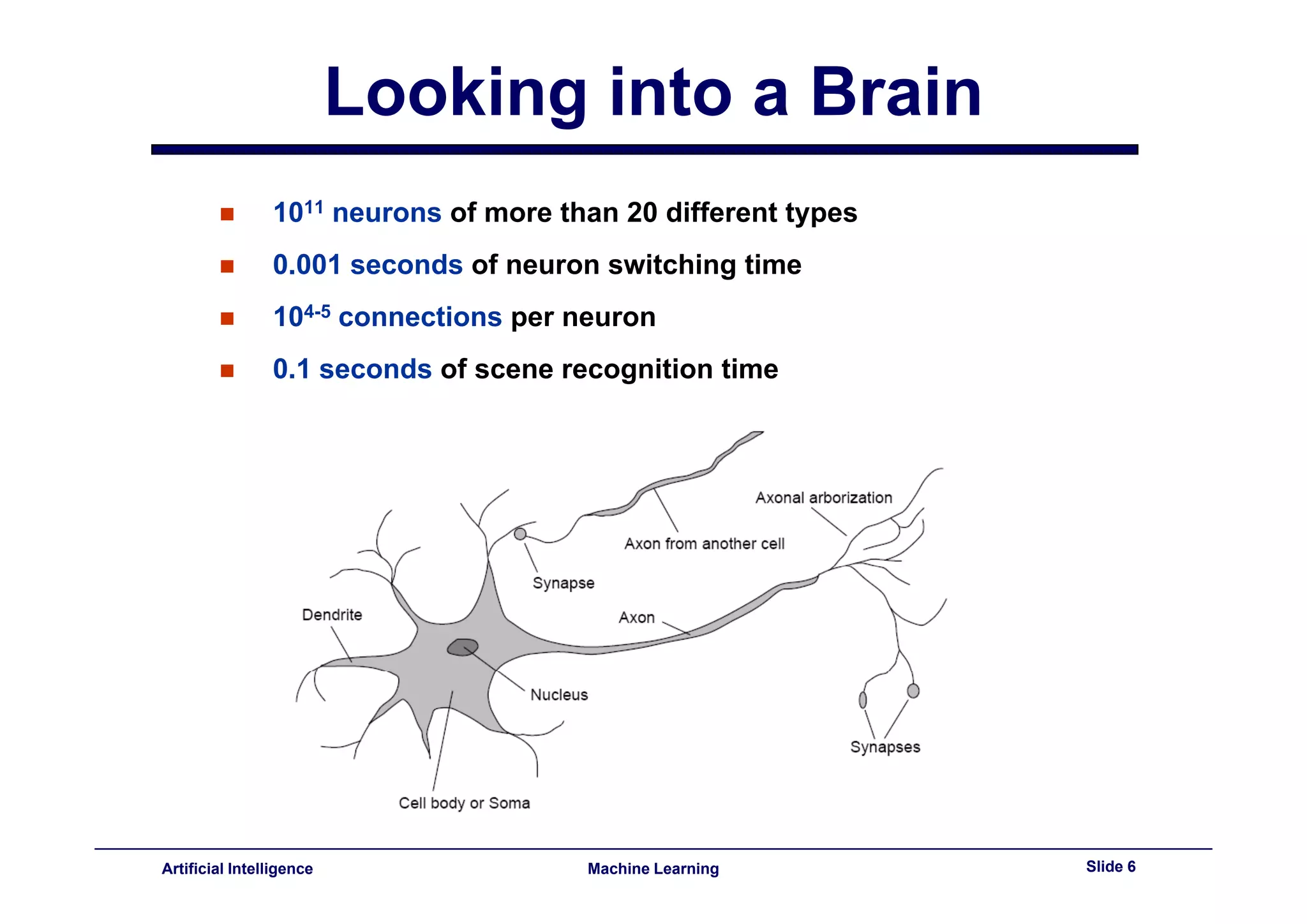
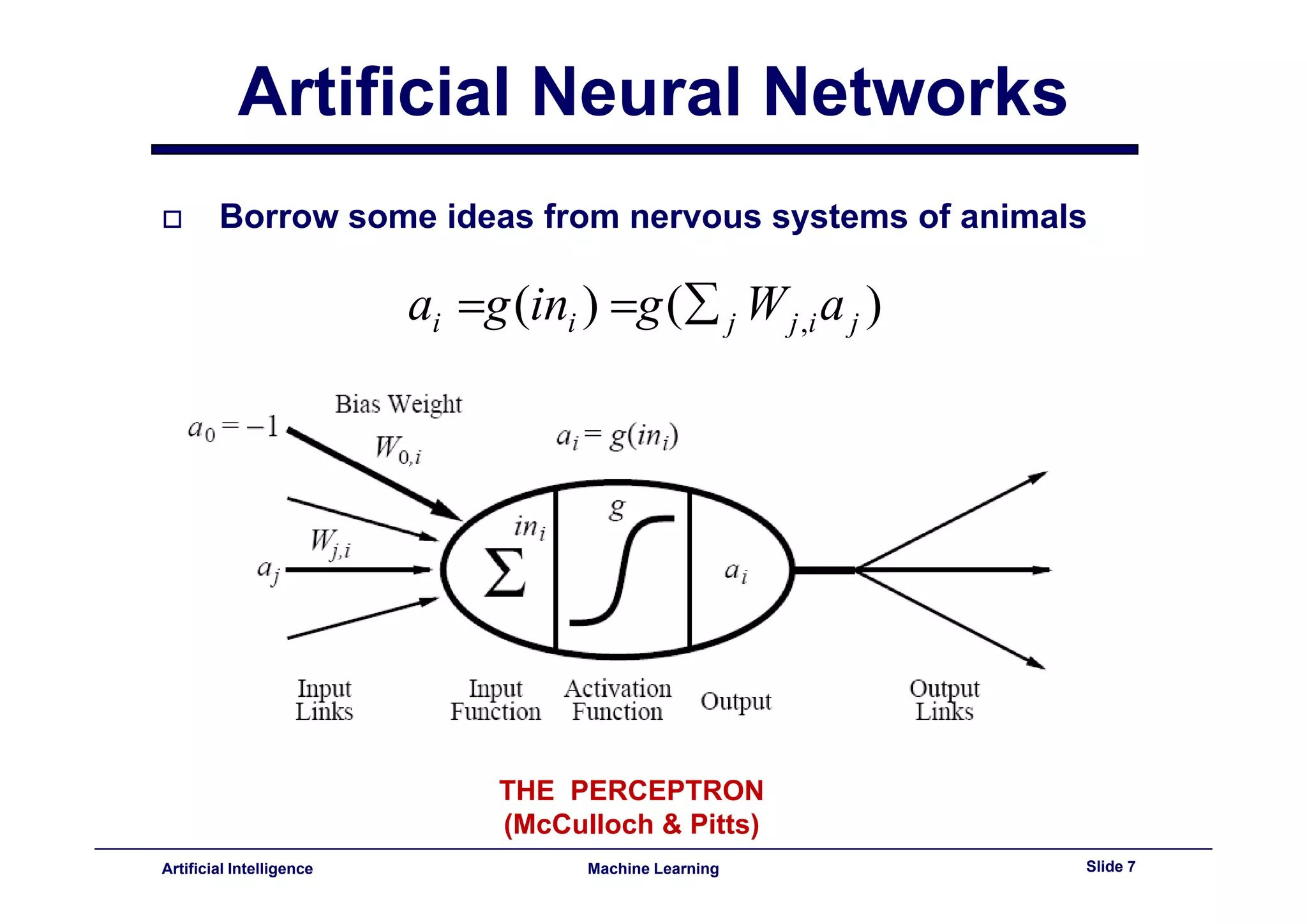
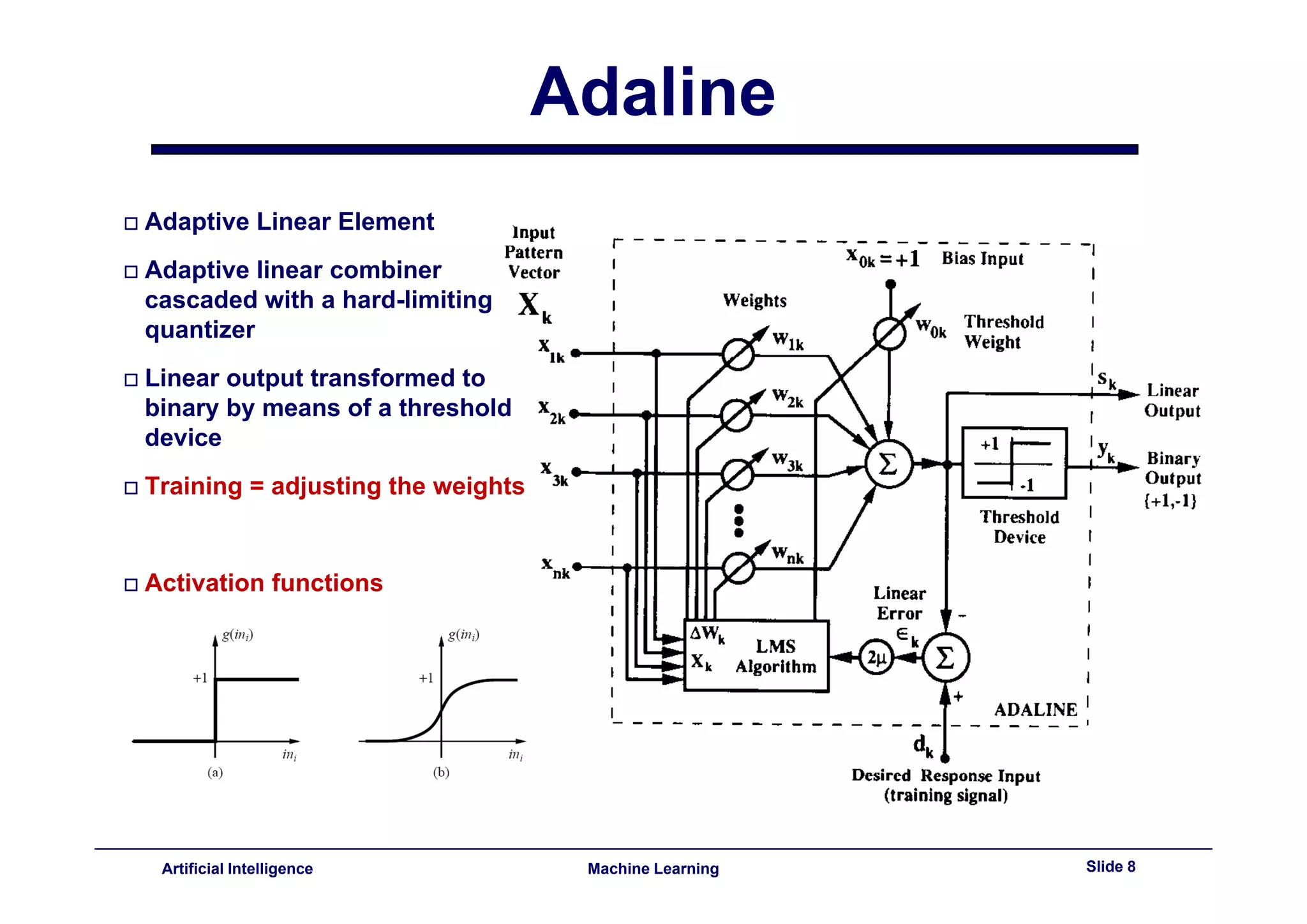
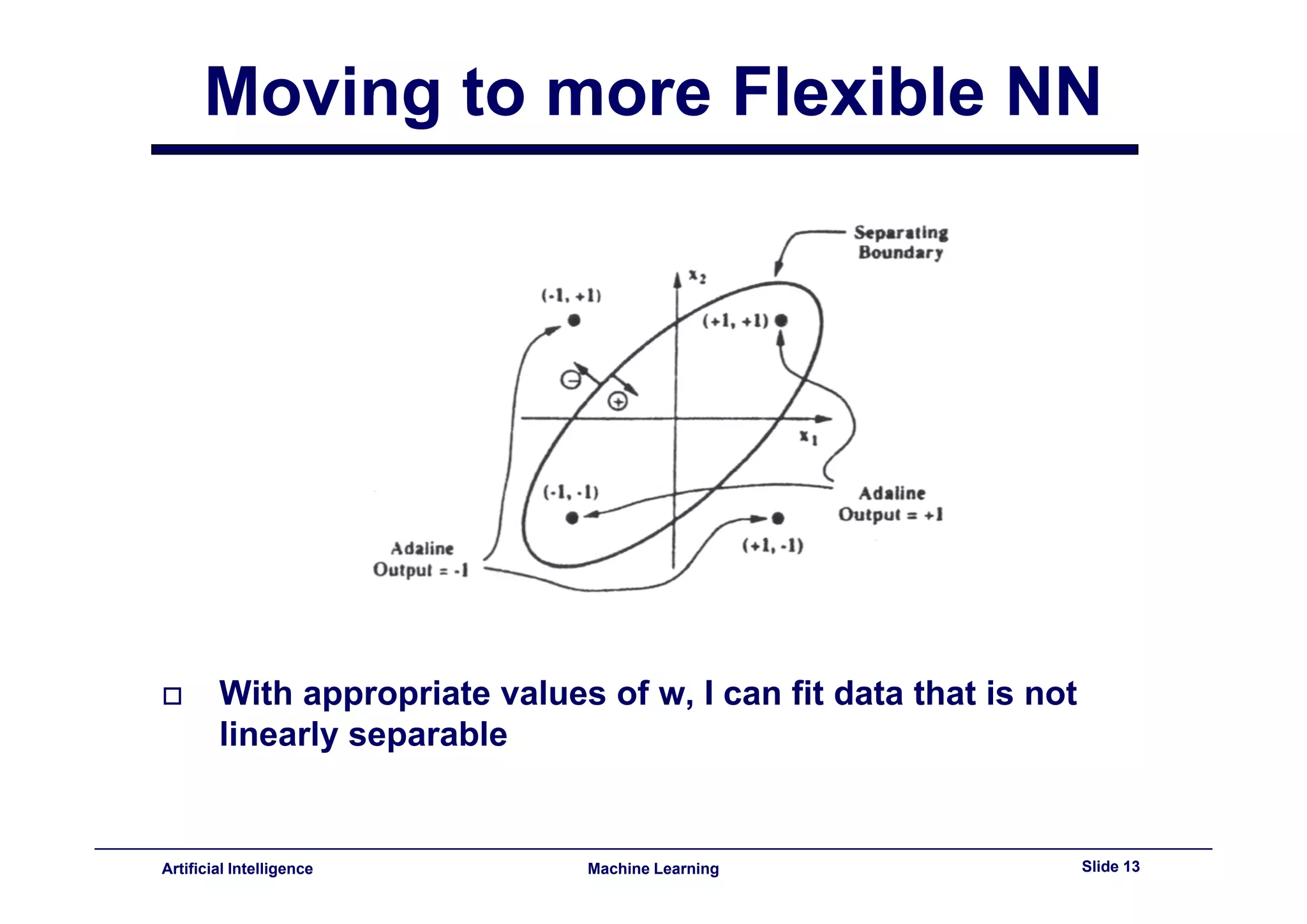
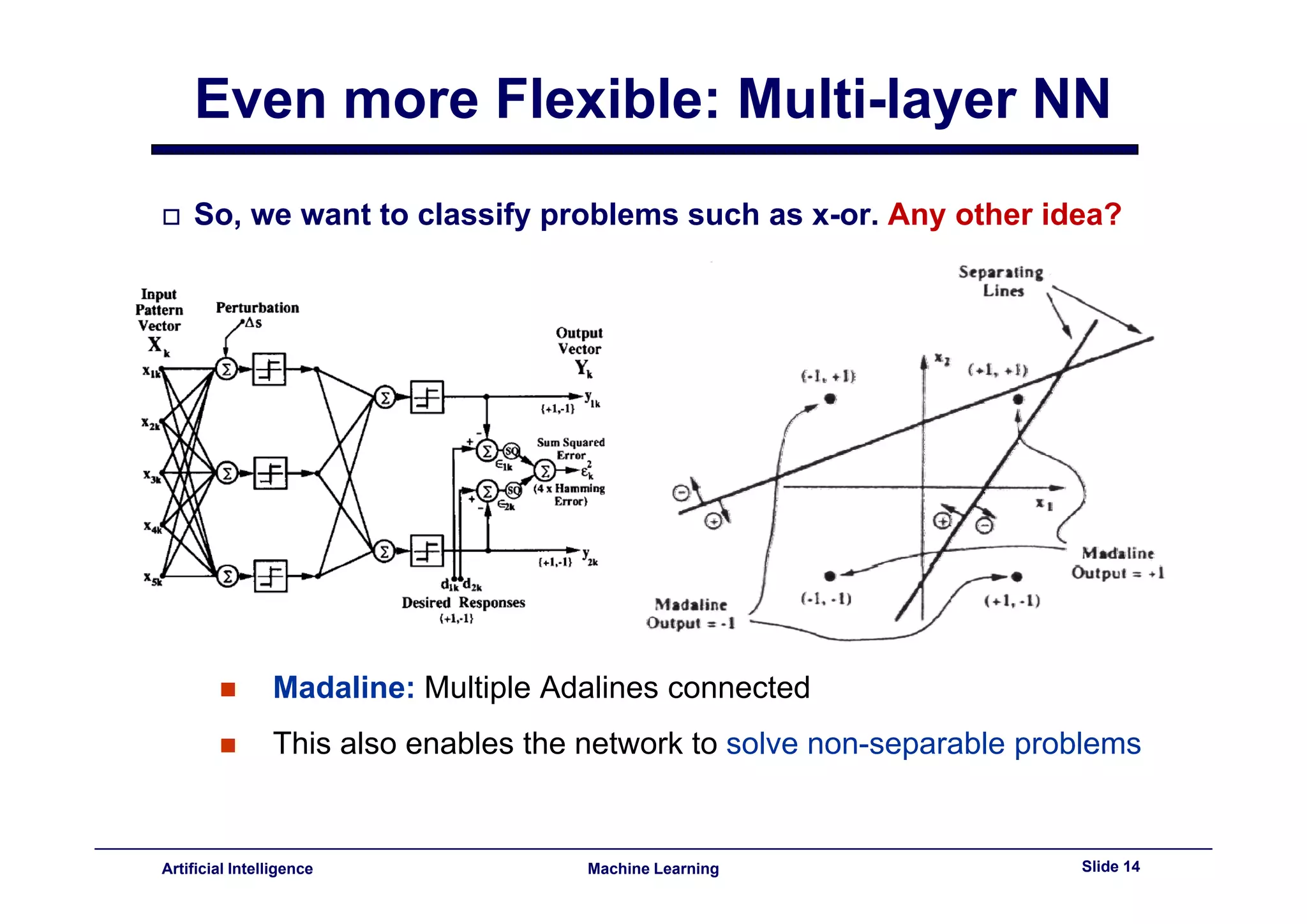
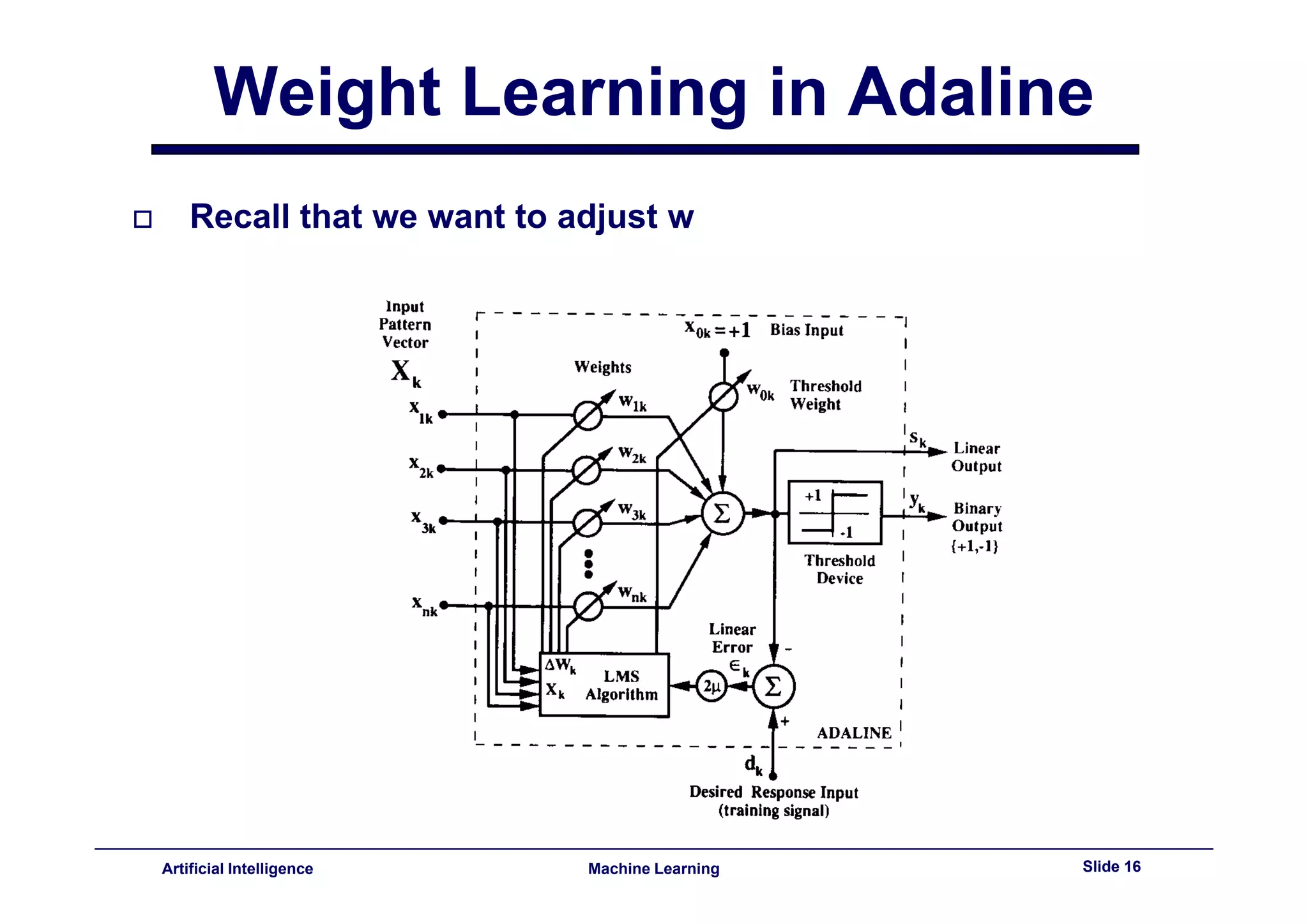
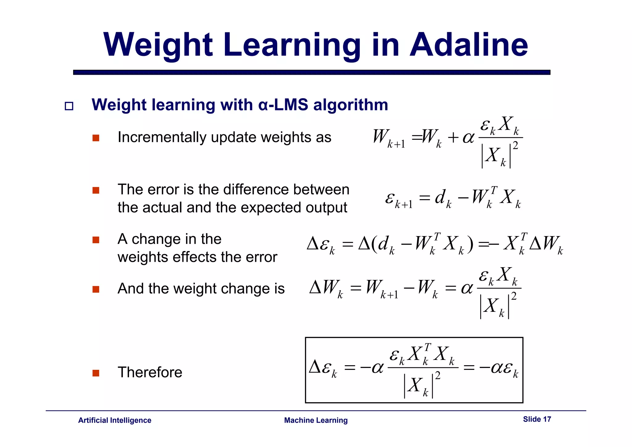
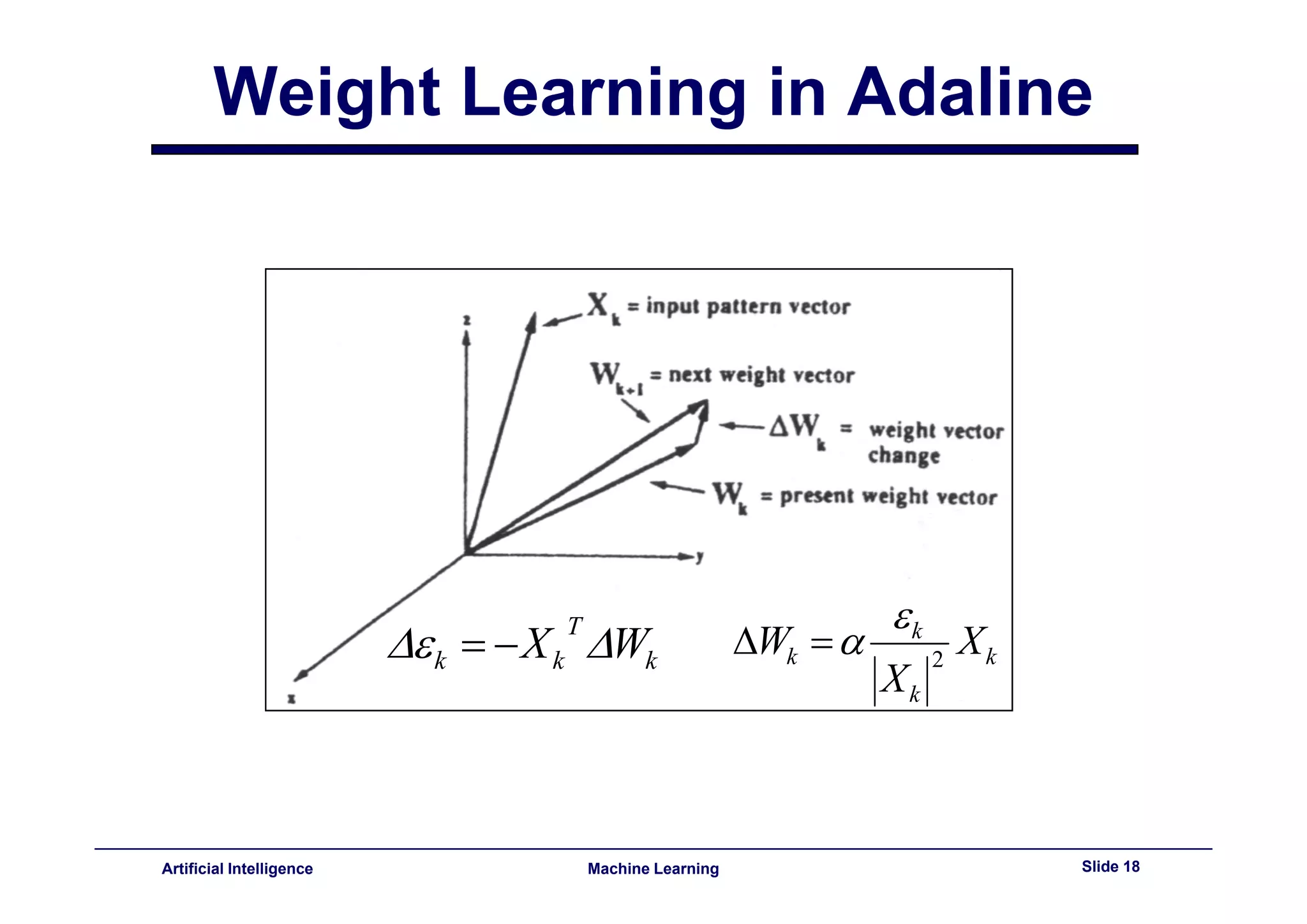
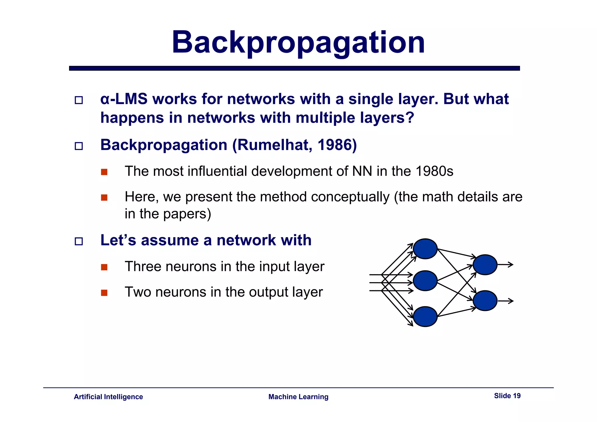
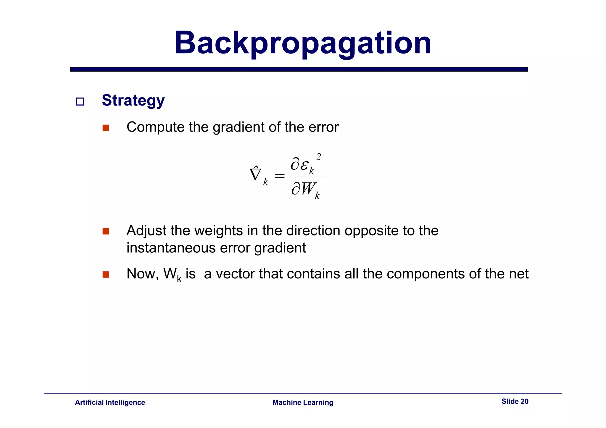
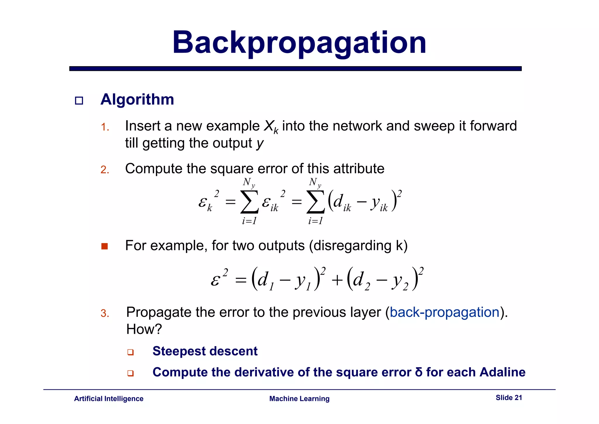
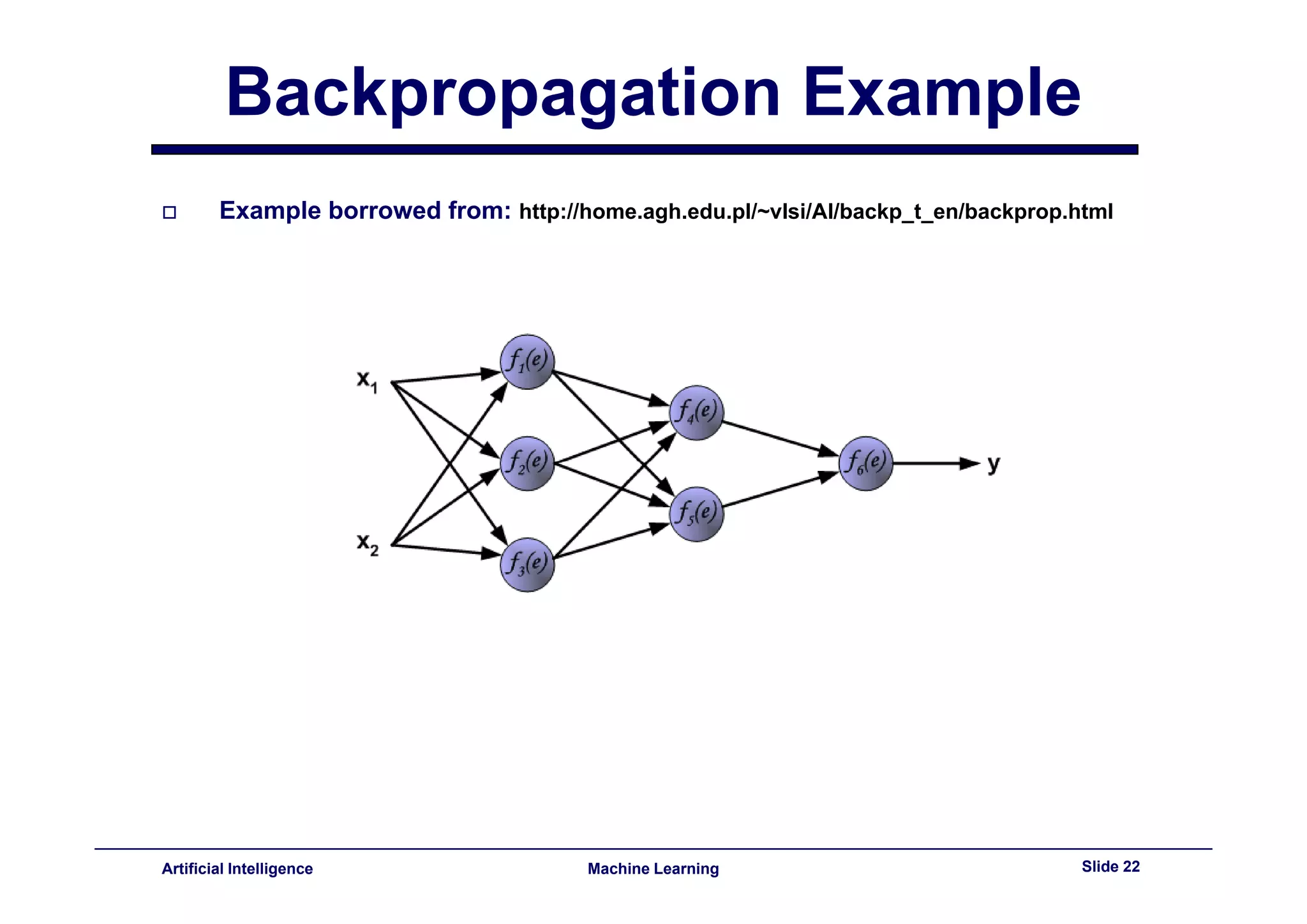
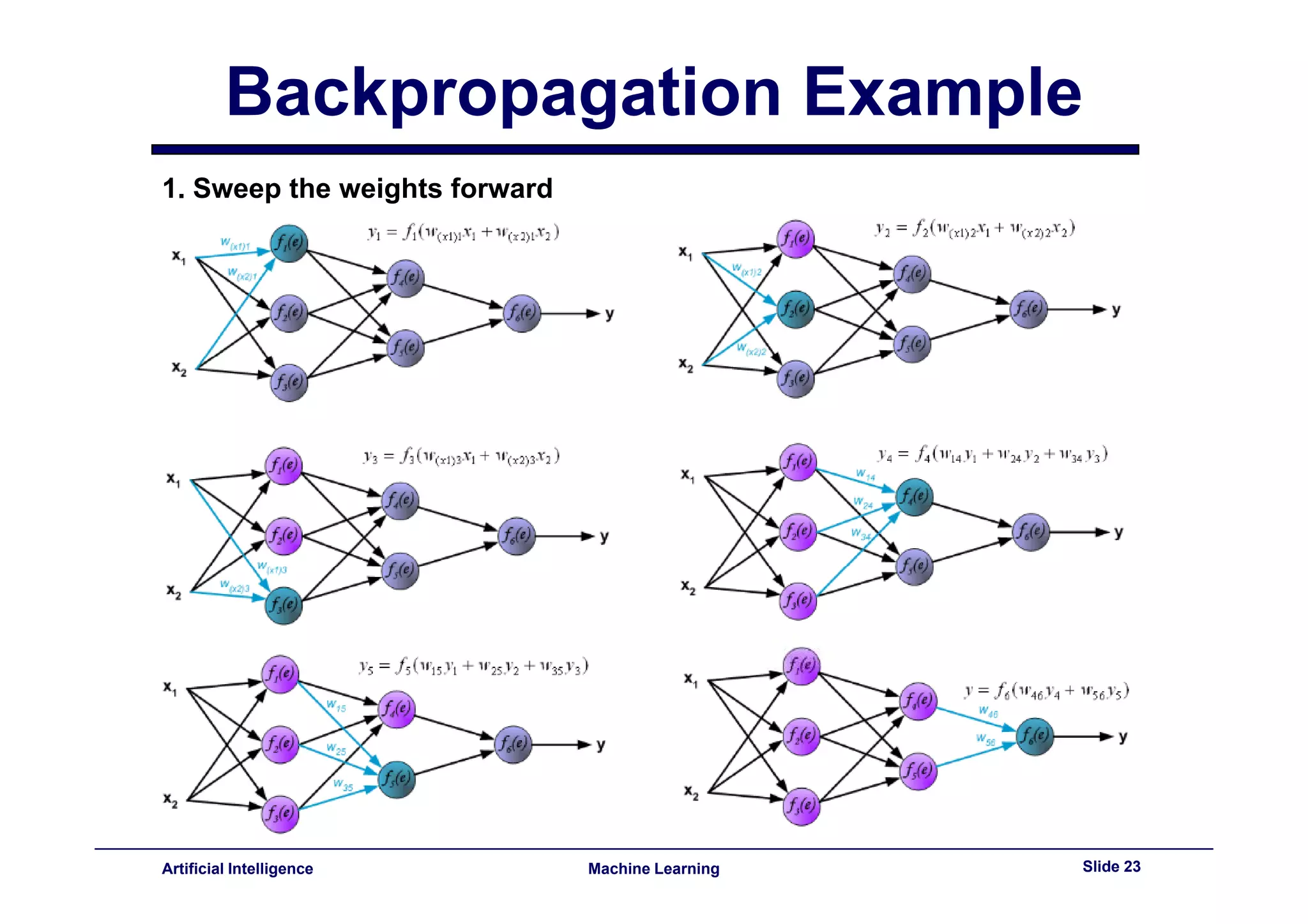
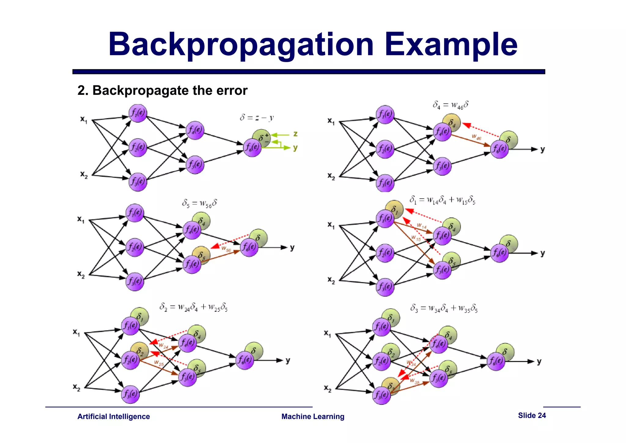
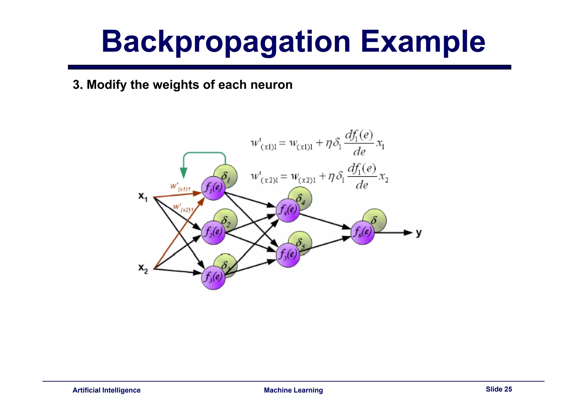
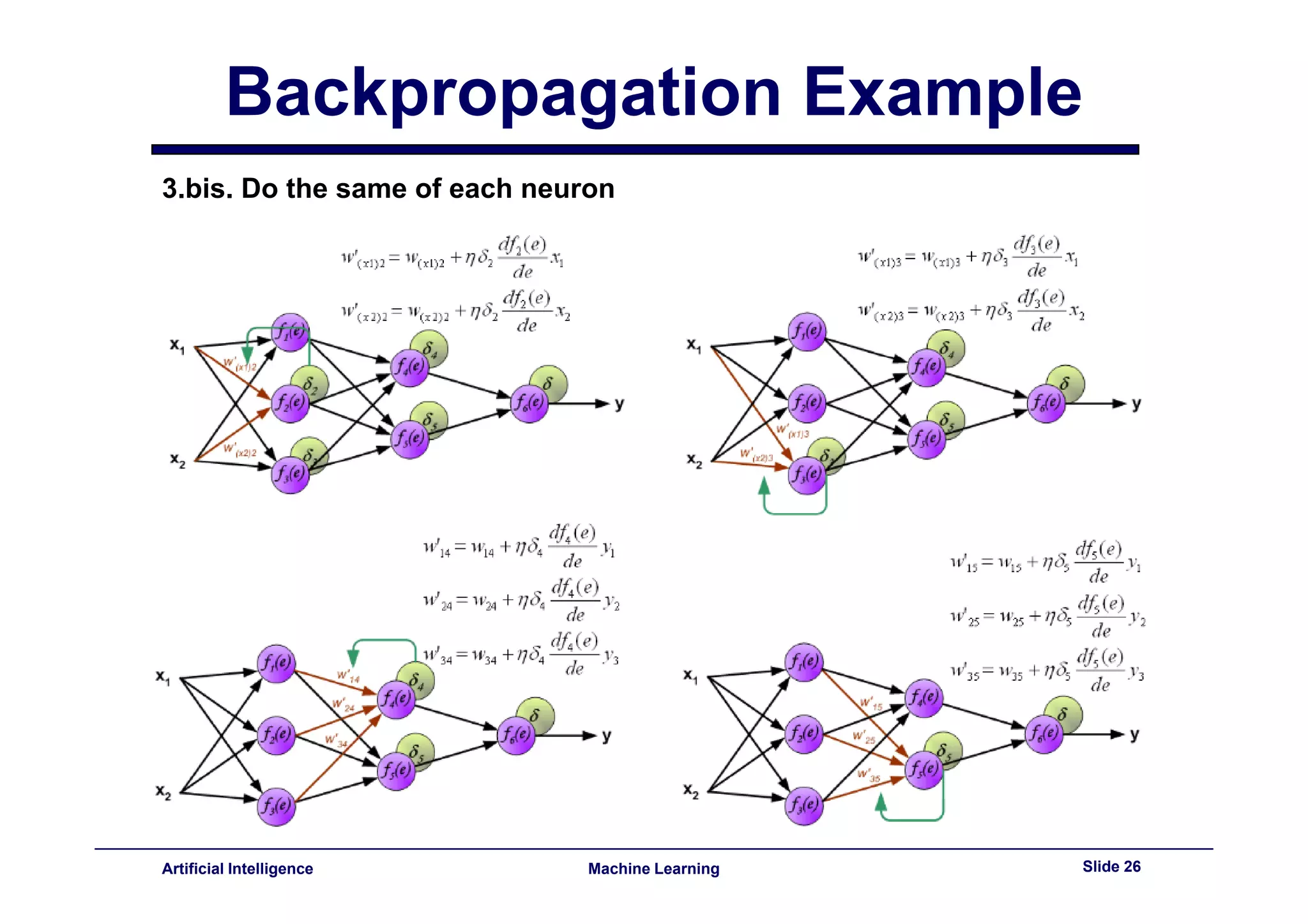
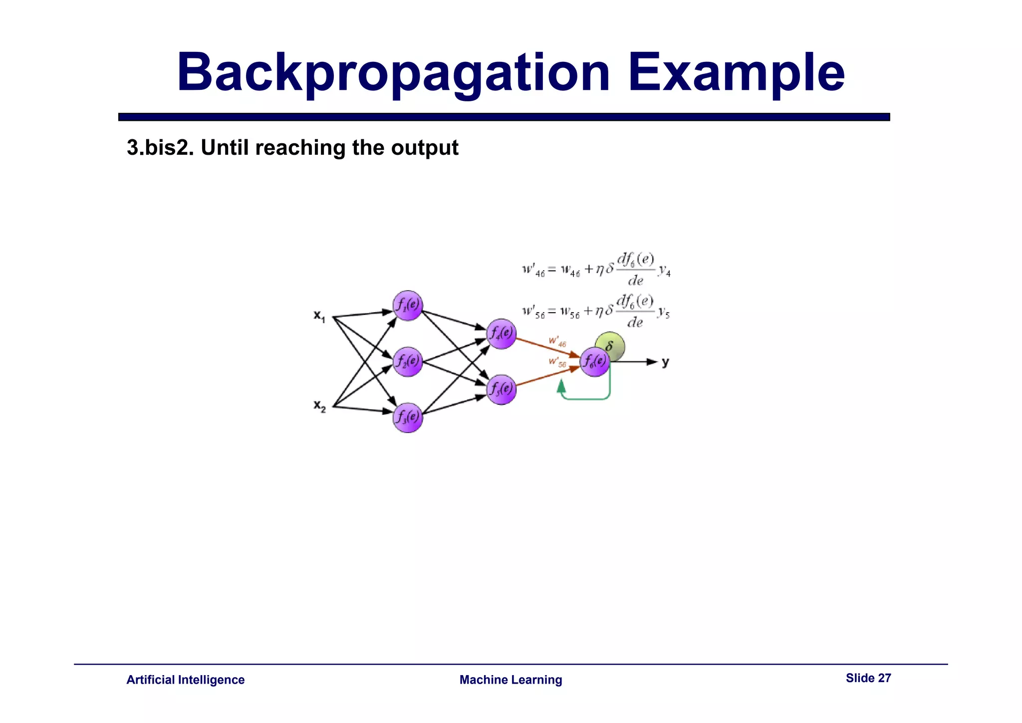
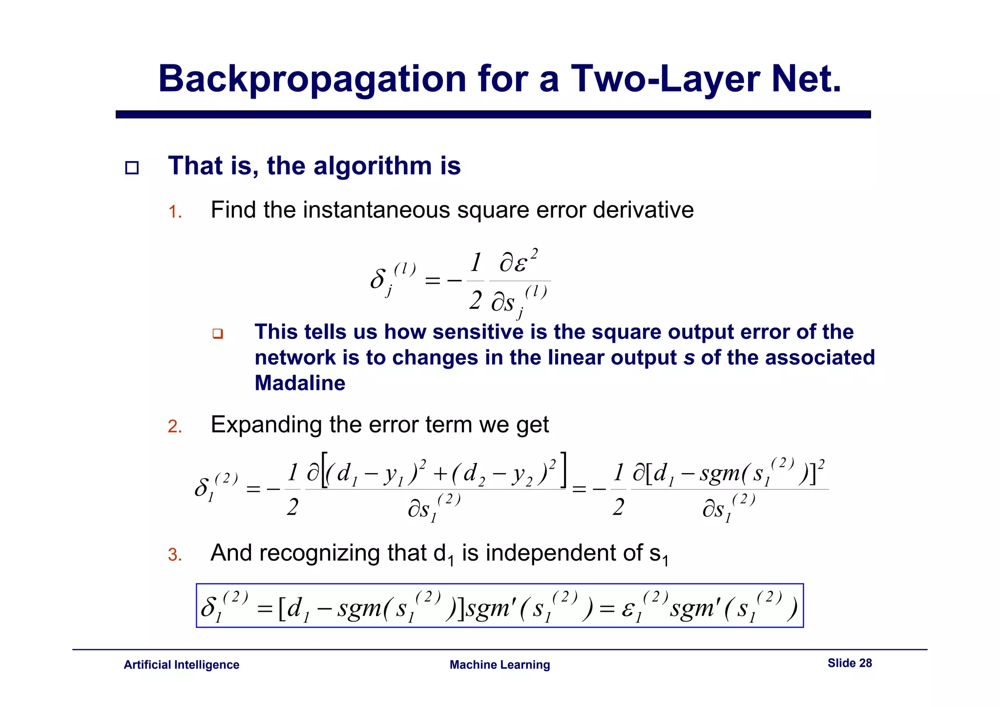

This document provides an overview of neural networks and backpropagation algorithms. It discusses how neural networks are inspired by biological brains and how they can be used to perform complex classification tasks. The key topics covered include perceptrons, Adaline networks, multi-layer perceptrons, backpropagation for training multi-layer networks, and an example of how backpropagation works to minimize error in a simple two-layer network.