This chapter analysis the two variable regression analysis

1. ADMAS UNIVERSITY
FACULTY of business and Economics
department of Economics
CHAPTER 2: TWO VARIABLE REGRESSION ANALYSIS:
SOME BASIC IDEAS
Senior Lecturer: Ahmed M. Elmi ( Atoshe)

2. A Hypothetical Example
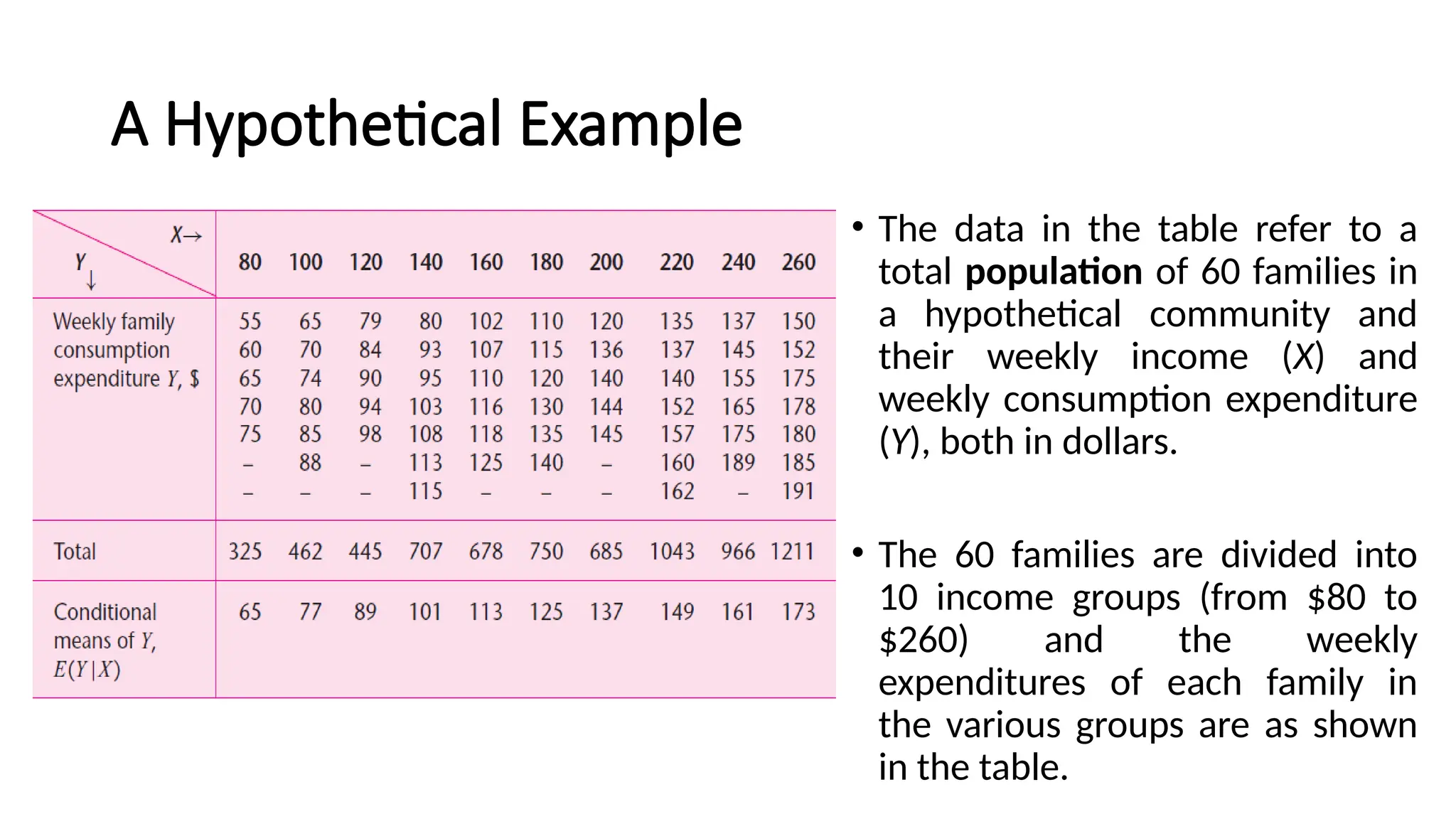
• The data in the table refer to a
total population of 60 families in
a hypothetical community and
their weekly income (X) and
weekly consumption expenditure
(Y), both in dollars.
• The 60 families are divided into
10 income groups (from $80 to
$260) and the weekly
expenditures of each family in
the various groups are as shown
in the table.

3. A Hypothetical Example
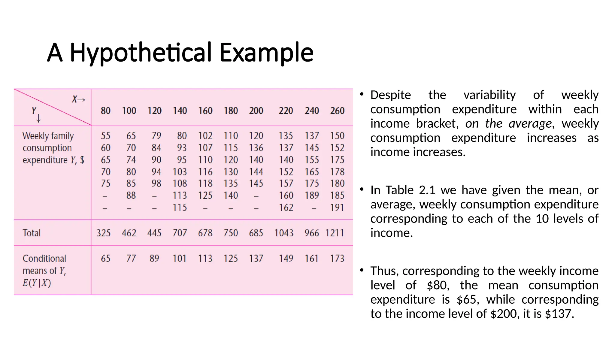
• Despite the variability of weekly
consumption expenditure within each
income bracket, on the average, weekly
consumption expenditure increases as
income increases.
• In Table 2.1 we have given the mean, or
average, weekly consumption expenditure
corresponding to each of the 10 levels of
income.
• Thus, corresponding to the weekly income
level of $80, the mean consumption
expenditure is $65, while corresponding
to the income level of $200, it is $137.

4. A Hypothetical Example
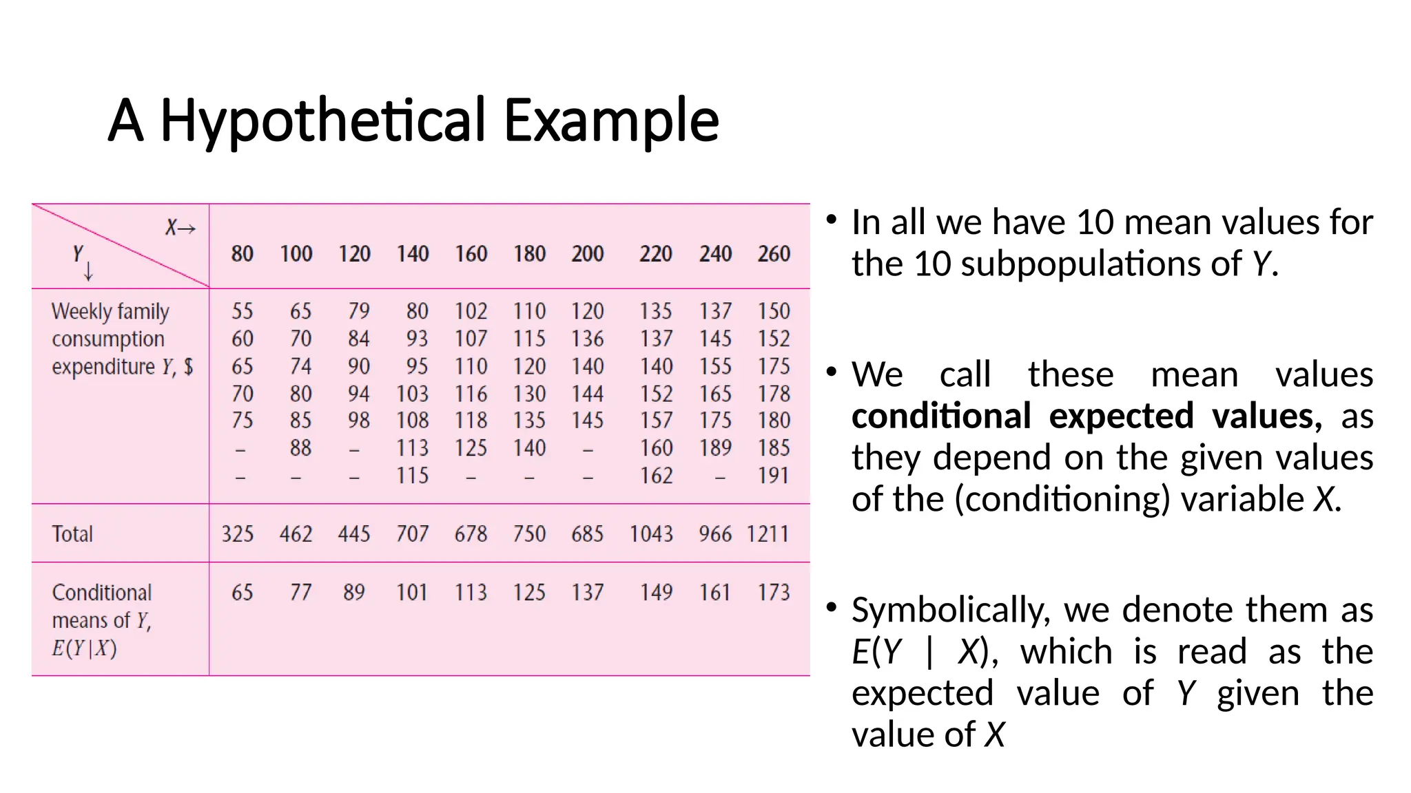
• In all we have 10 mean values for
the 10 subpopulations of Y.
• We call these mean values
conditional expected values, as
they depend on the given values
of the (conditioning) variable X.
• Symbolically, we denote them as
E(Y | X), which is read as the
expected value of Y given the
value of X

5. A Hypothetical Example
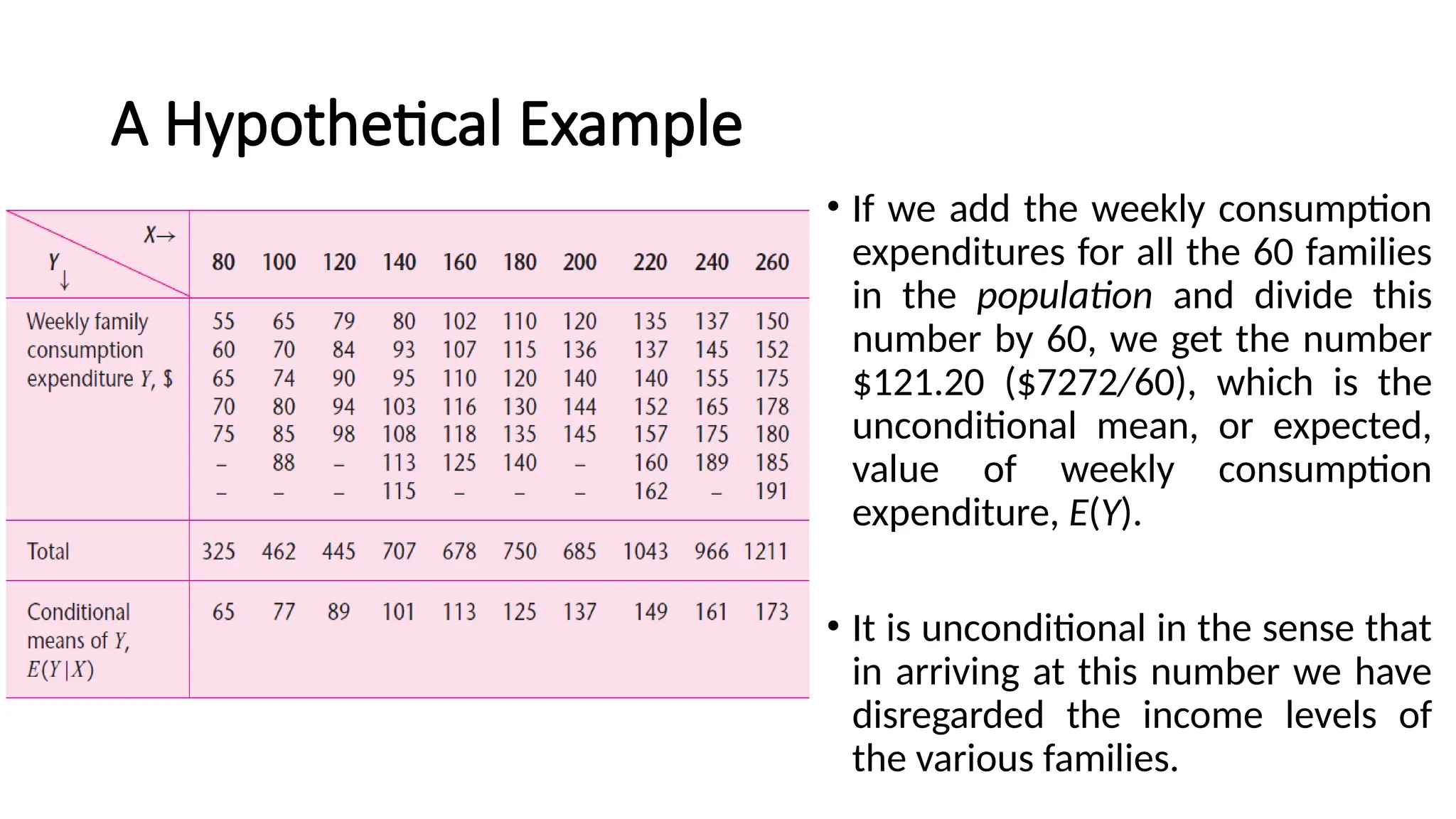
• If we add the weekly consumption
expenditures for all the 60 families
in the population and divide this
number by 60, we get the number
$121.20 ($7272/60), which is the
unconditional mean, or expected,
value of weekly consumption
expenditure, E(Y).
• It is unconditional in the sense that
in arriving at this number we have
disregarded the income levels of
the various families.

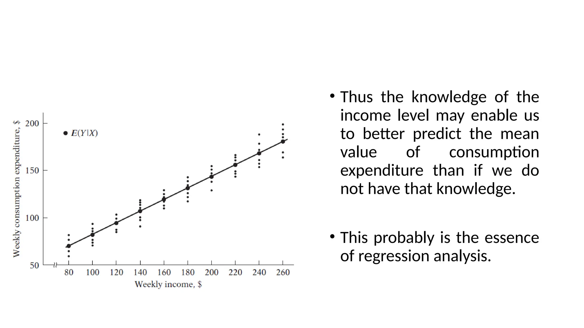
6. • Thus the knowledge of the
income level may enable us
to better predict the mean
value of consumption
expenditure than if we do
not have that knowledge.
• This probably is the essence
of regression analysis.

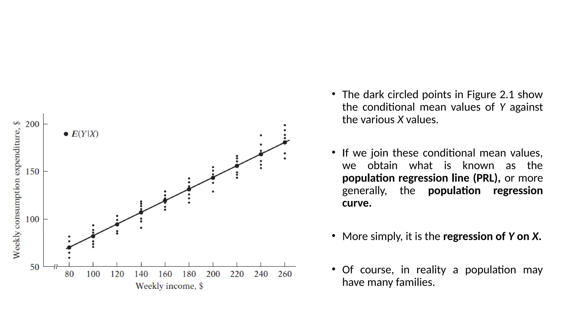
7. • The dark circled points in Figure 2.1 show
the conditional mean values of Y against
the various X values.
• If we join these conditional mean values,
we obtain what is known as the
population regression line (PRL), or more
generally, the population regression
curve.
• More simply, it is the regression of Y on X.
• Of course, in reality a population may
have many families.

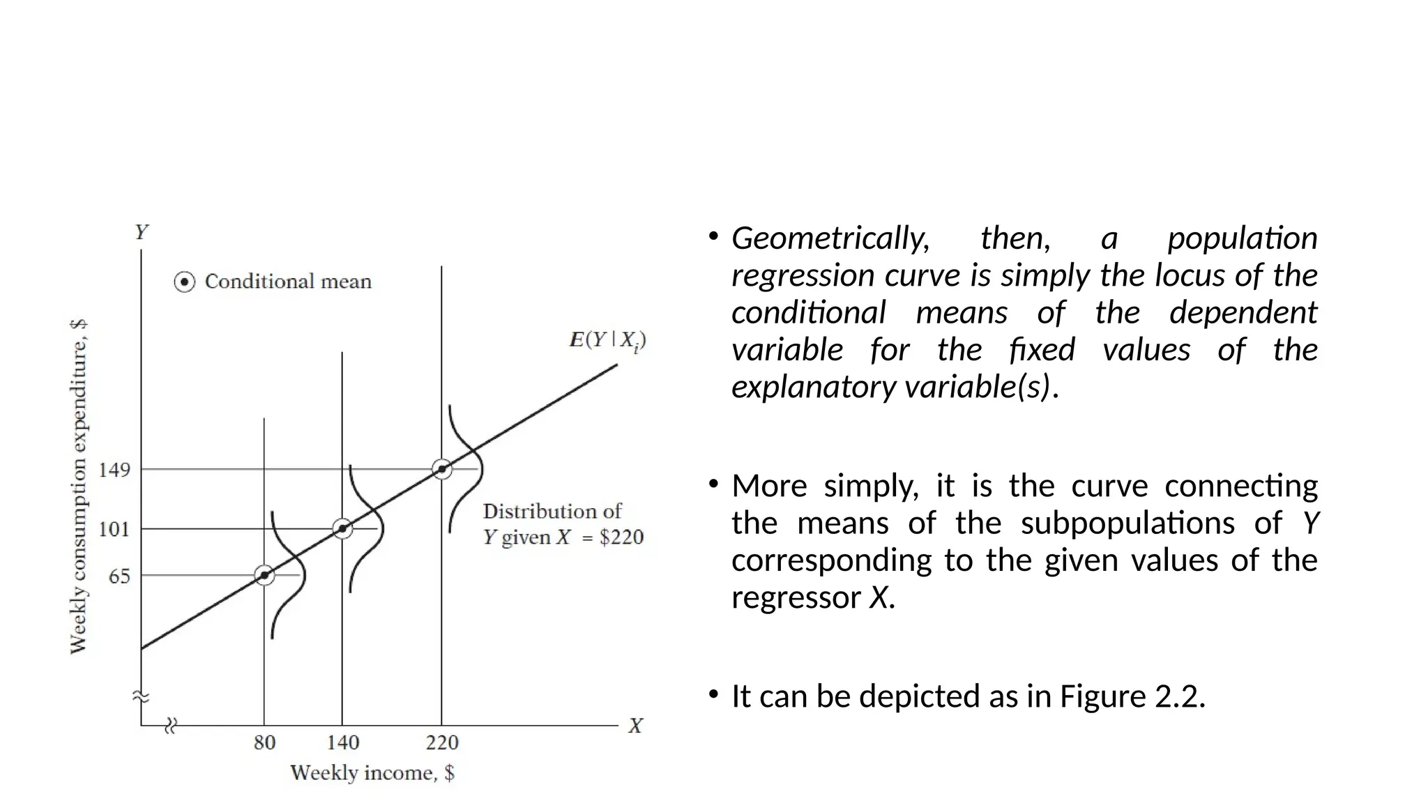
8. • Geometrically, then, a population
regression curve is simply the locus of the
conditional means of the dependent
variable for the fixed values of the
explanatory variable(s).
• More simply, it is the curve connecting
the means of the subpopulations of Y
corresponding to the given values of the
regressor X.
• It can be depicted as in Figure 2.2.

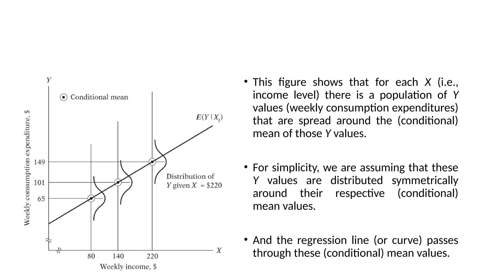
9. • This figure shows that for each X (i.e.,
income level) there is a population of Y
values (weekly consumption expenditures)
that are spread around the (conditional)
mean of those Y values.
• For simplicity, we are assuming that these
Y values are distributed symmetrically
around their respective (conditional)
mean values.
• And the regression line (or curve) passes
through these (conditional) mean values.

10. The Concept of Population Regression
Function (PRF)
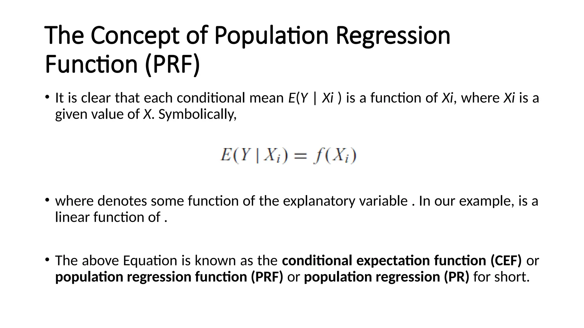
• It is clear that each conditional mean E(Y | Xi ) is a function of Xi, where Xi is a
given value of X. Symbolically,
• where denotes some function of the explanatory variable . In our example, is a
linear function of .
• The above Equation is known as the conditional expectation function (CEF) or
population regression function (PRF) or population regression (PR) for short.

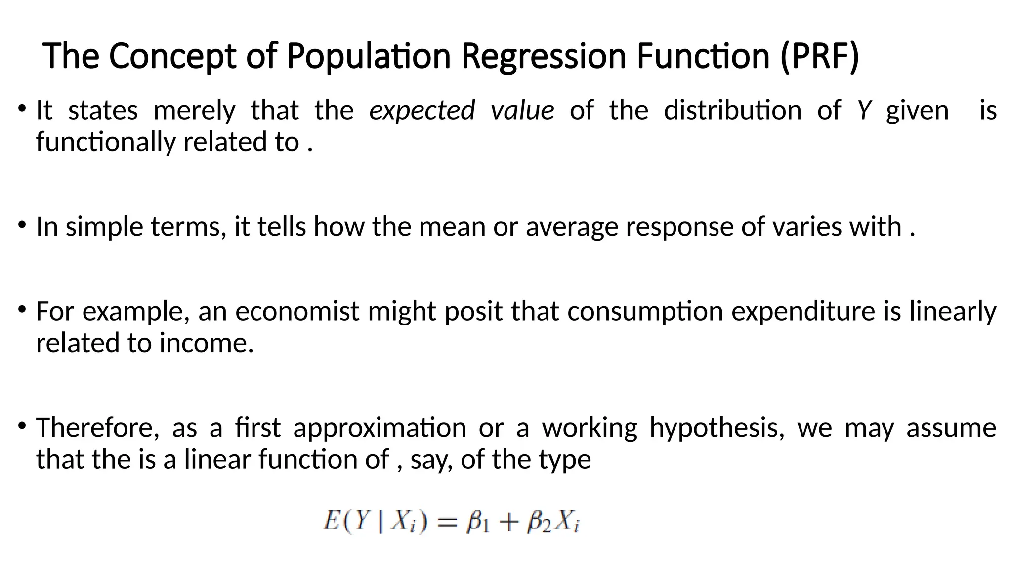
11. • It states merely that the expected value of the distribution of Y given is
functionally related to .
• In simple terms, it tells how the mean or average response of varies with .
• For example, an economist might posit that consumption expenditure is linearly
related to income.
• Therefore, as a first approximation or a working hypothesis, we may assume
that the is a linear function of , say, of the type
The Concept of Population Regression Function (PRF)

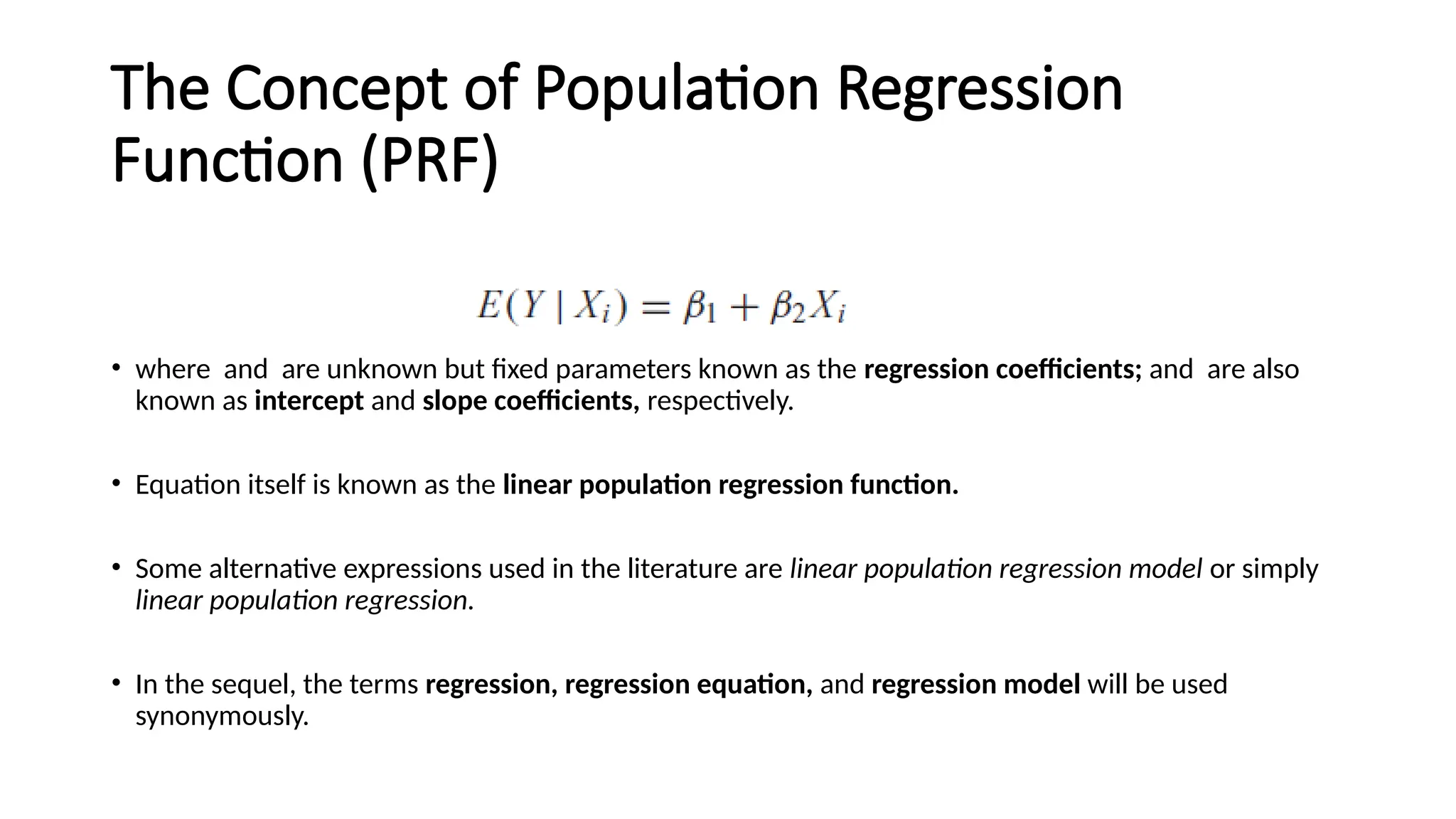
12. • where and are unknown but fixed parameters known as the regression coefficients; and are also
known as intercept and slope coefficients, respectively.
• Equation itself is known as the linear population regression function.
• Some alternative expressions used in the literature are linear population regression model or simply
linear population regression.
• In the sequel, the terms regression, regression equation, and regression model will be used
synonymously.
The Concept of Population Regression
Function (PRF)

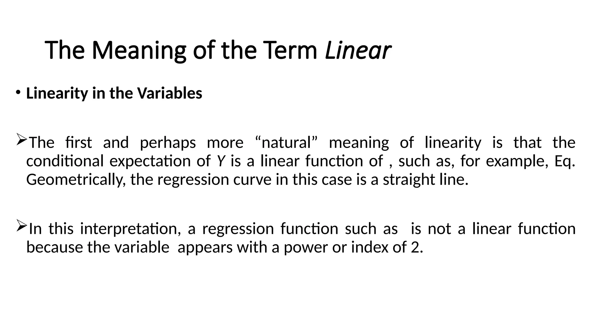
13. The Meaning of the Term Linear
• Linearity in the Variables
The first and perhaps more “natural” meaning of linearity is that the
conditional expectation of Y is a linear function of , such as, for example, Eq.
Geometrically, the regression curve in this case is a straight line.
In this interpretation, a regression function such as is not a linear function
because the variable appears with a power or index of 2.

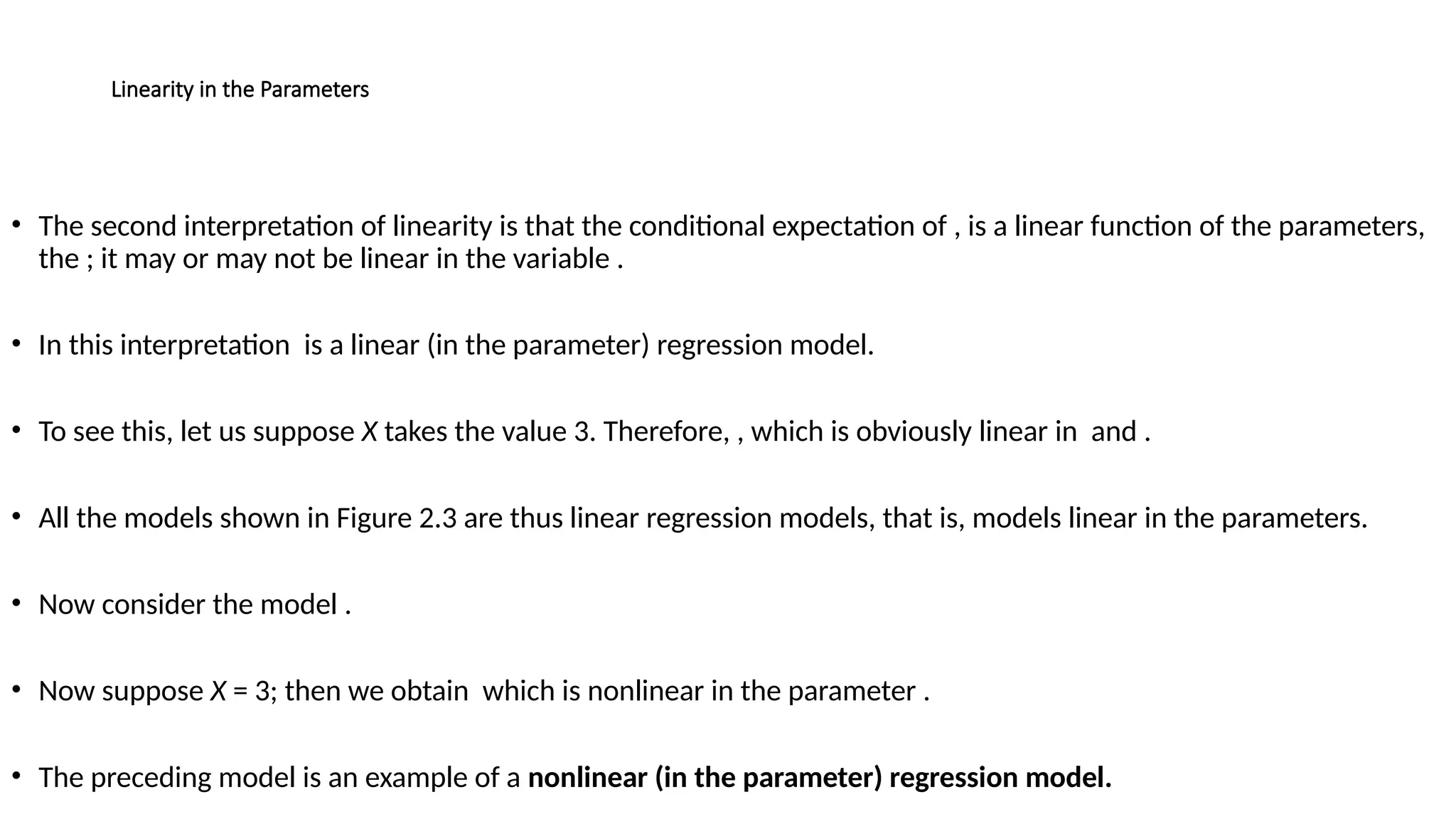
14. Linearity in the Parameters
• The second interpretation of linearity is that the conditional expectation of , is a linear function of the parameters,
the ; it may or may not be linear in the variable .
• In this interpretation is a linear (in the parameter) regression model.
• To see this, let us suppose X takes the value 3. Therefore, , which is obviously linear in and .
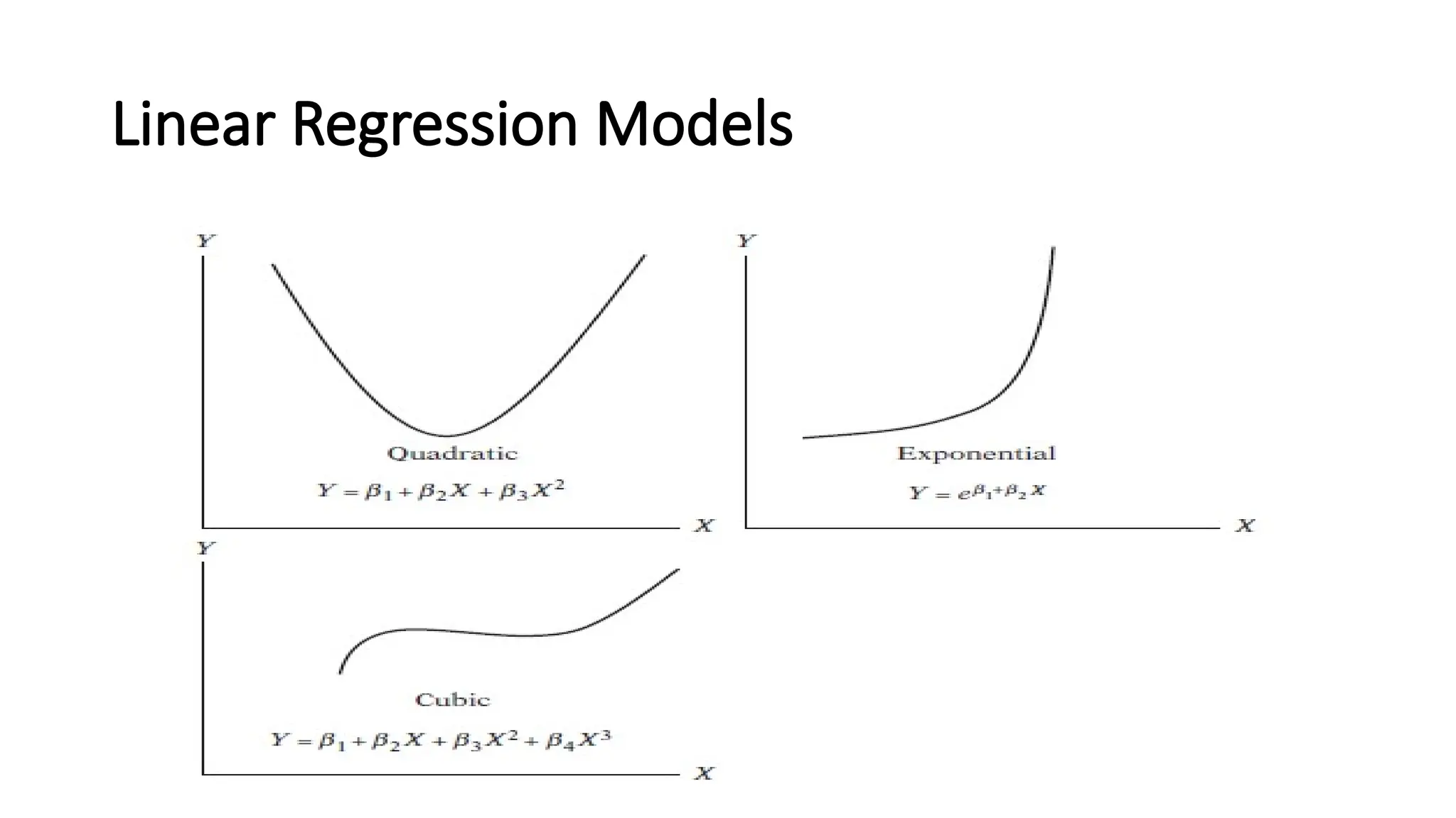
• All the models shown in Figure 2.3 are thus linear regression models, that is, models linear in the parameters.
• Now consider the model .
• Now suppose X = 3; then we obtain which is nonlinear in the parameter .
• The preceding model is an example of a nonlinear (in the parameter) regression model.

15. • The term “linear” regression will always mean a regression that is linear in
the parameters; the (that is, the parameters) are raised to the first power
only.
• It may or may not be linear in the explanatory variables, the .
• Thus, which is linear both in the parameters and variable, is a LRM.
• , which is linear in the parameters but nonlinear in variable X.
Linearity in the Parameters

16. Linear Regression Models

17. Stochastic Specification of PRF
• As family income increases, family consumption expenditure on the
average increases, too.
• But what about the consumption expenditure of an individual family
in relation to its (fixed) level of income?
• An individual family’s consumption expenditure does not necessarily
increase as the income level increases.

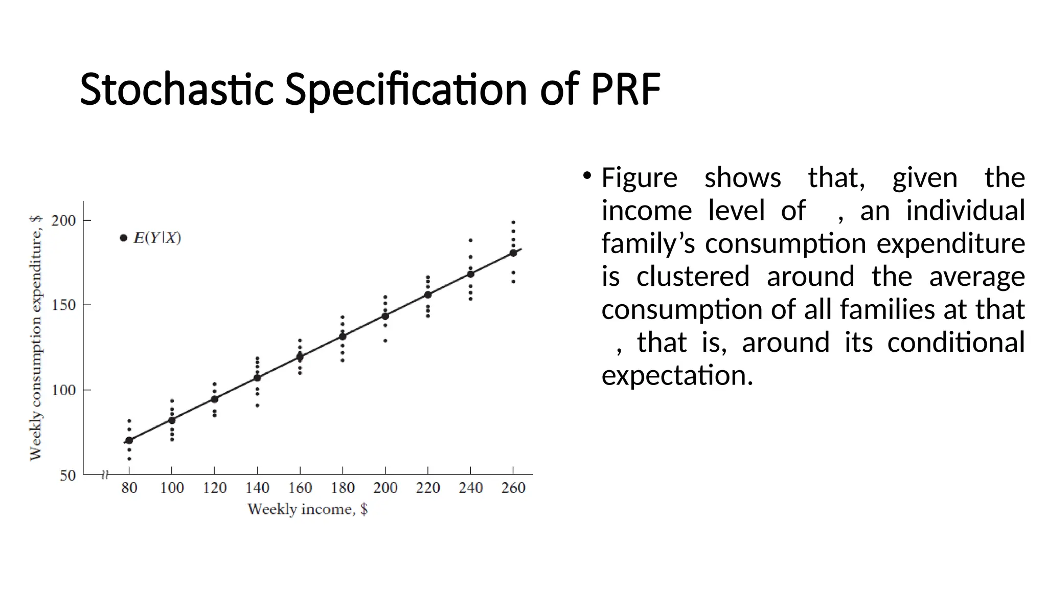
18. • Figure shows that, given the
income level of , an individual
family’s consumption expenditure
is clustered around the average
consumption of all families at that
, that is, around its conditional
expectation.
Stochastic Specification of PRF

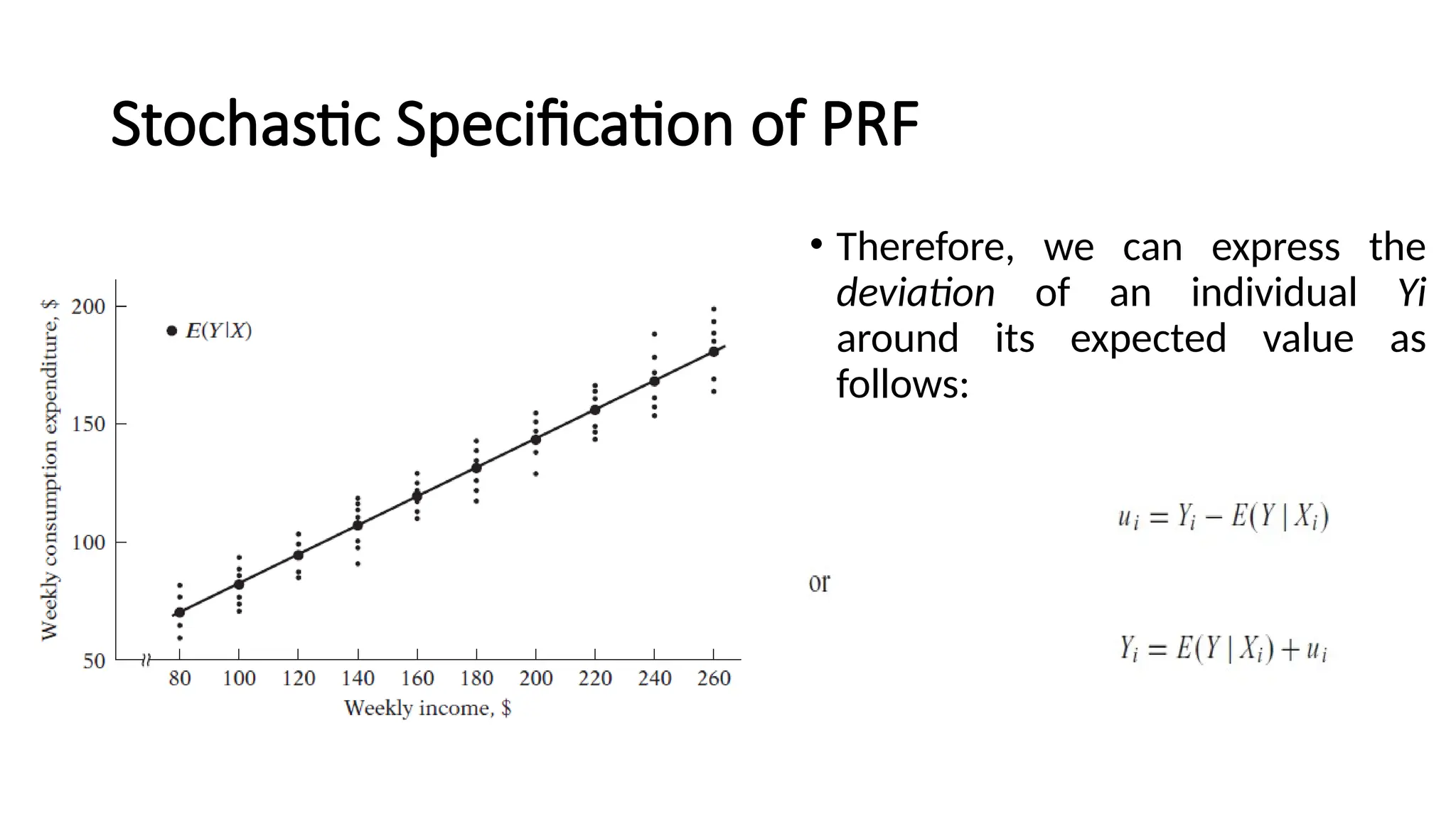
19. • Therefore, we can express the
deviation of an individual Yi
around its expected value as
follows:
Stochastic Specification of PRF

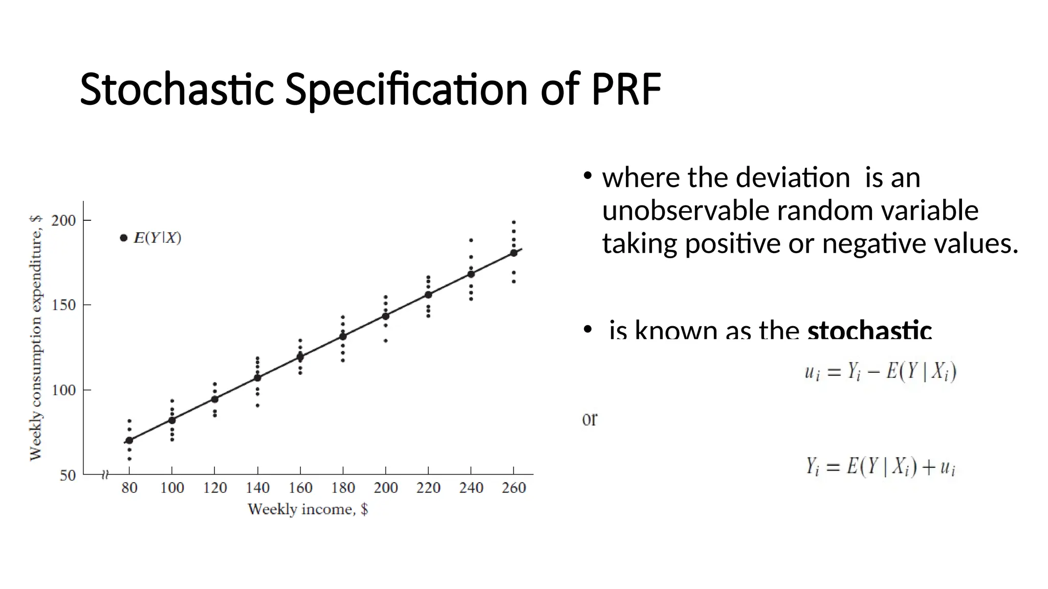
20. • where the deviation is an
unobservable random variable
taking positive or negative values.
• is known as the stochastic
disturbance or stochastic error
term.
Stochastic Specification of PRF

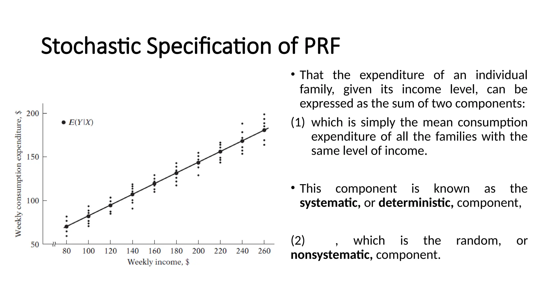
21. • That the expenditure of an individual
family, given its income level, can be
expressed as the sum of two components:
(1) which is simply the mean consumption
expenditure of all the families with the
same level of income.
• This component is known as the
systematic, or deterministic, component,
(2) , which is the random, or
nonsystematic, component.
Stochastic Specification of PRF

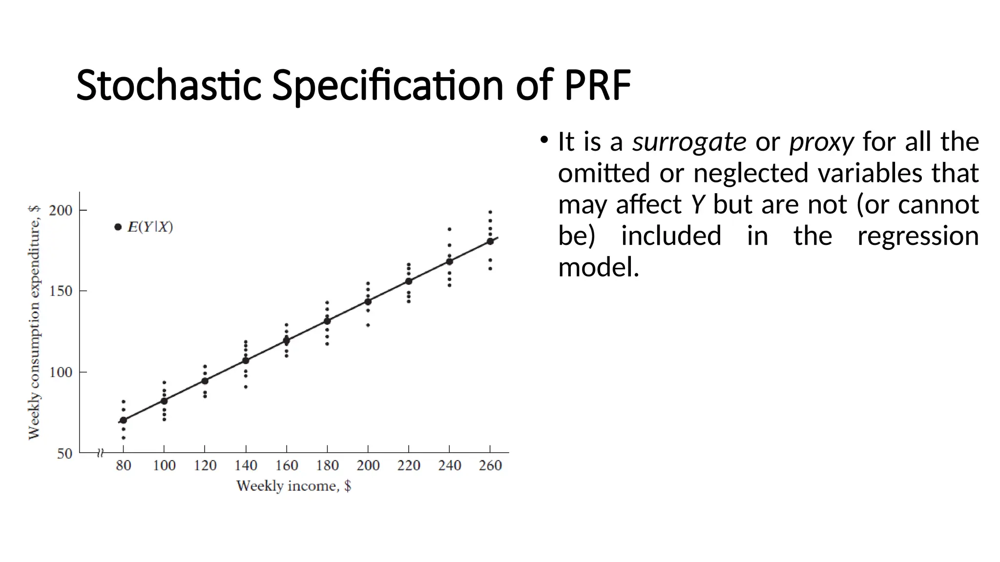
22. • It is a surrogate or proxy for all the
omitted or neglected variables that
may affect Y but are not (or cannot
be) included in the regression
model.
Stochastic Specification of PRF

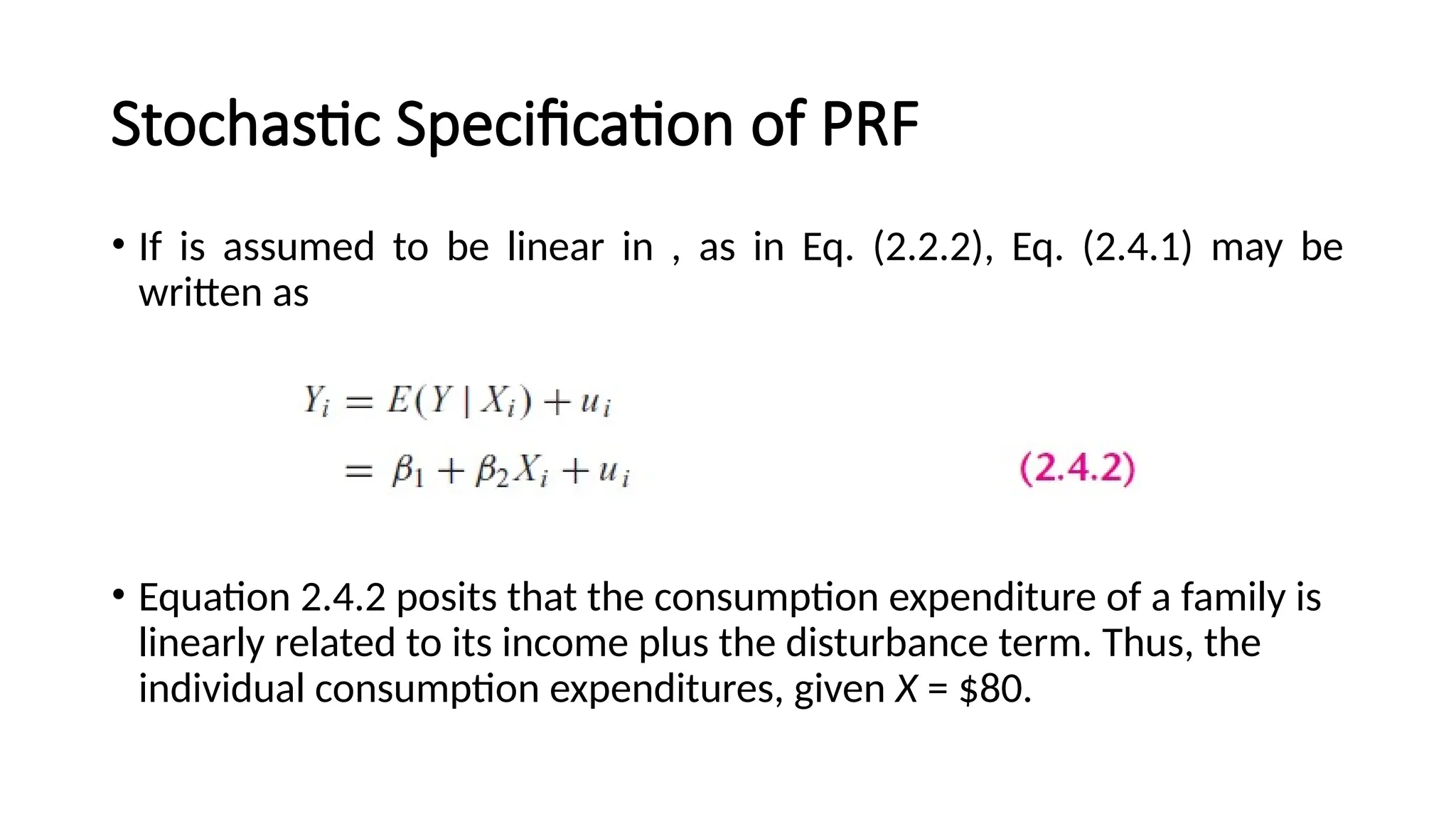
23. • If is assumed to be linear in , as in Eq. (2.2.2), Eq. (2.4.1) may be
written as
• Equation 2.4.2 posits that the consumption expenditure of a family is
linearly related to its income plus the disturbance term. Thus, the
individual consumption expenditures, given X = $80.
Stochastic Specification of PRF

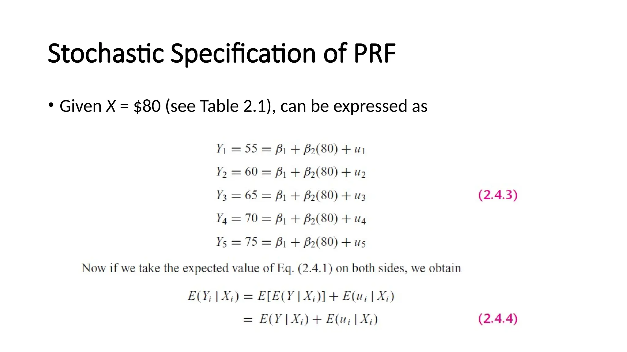
24. • Given X = $80 (see Table 2.1), can be expressed as
Stochastic Specification of PRF

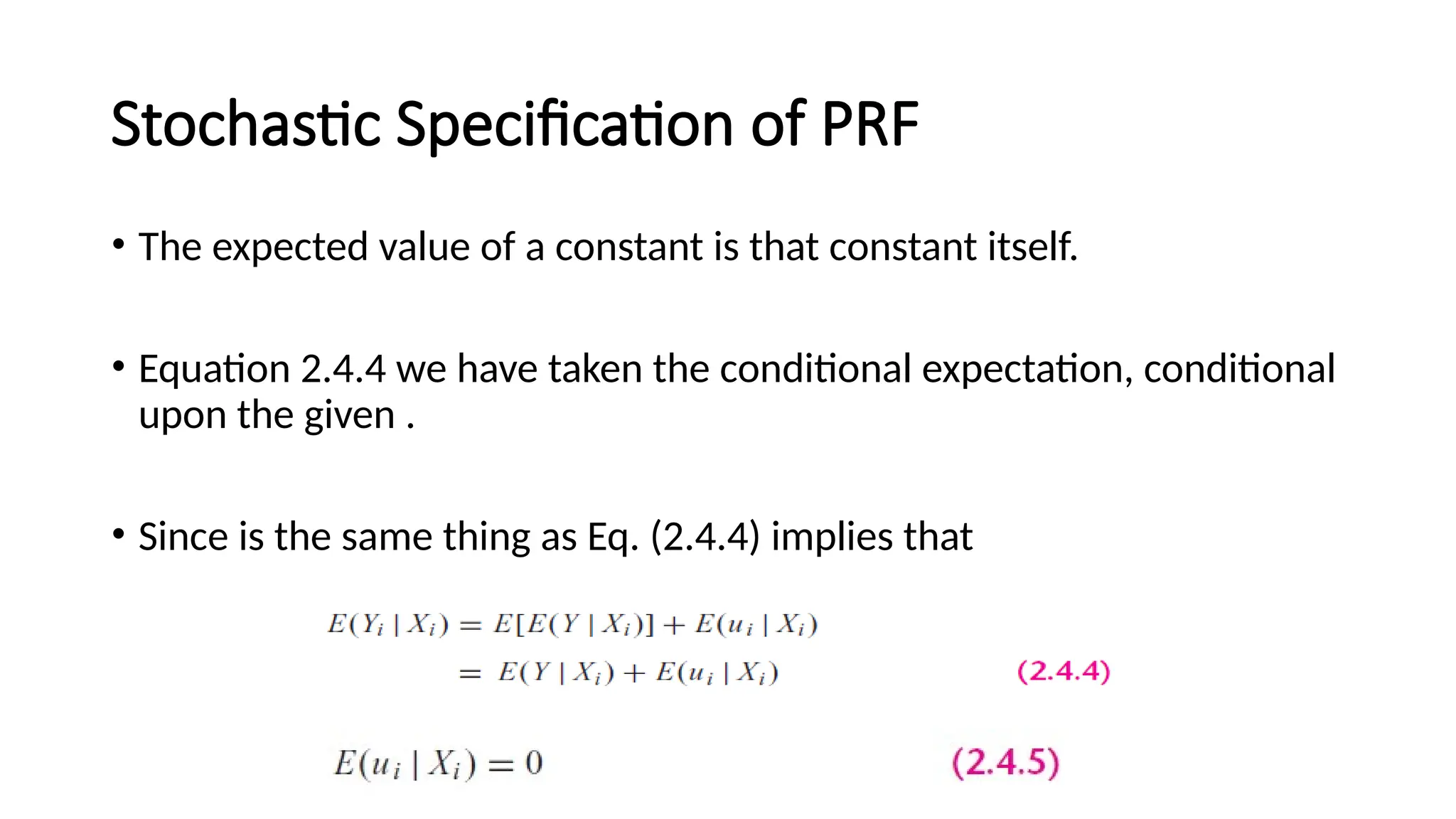
25. • The expected value of a constant is that constant itself.
• Equation 2.4.4 we have taken the conditional expectation, conditional
upon the given .
• Since is the same thing as Eq. (2.4.4) implies that
Stochastic Specification of PRF

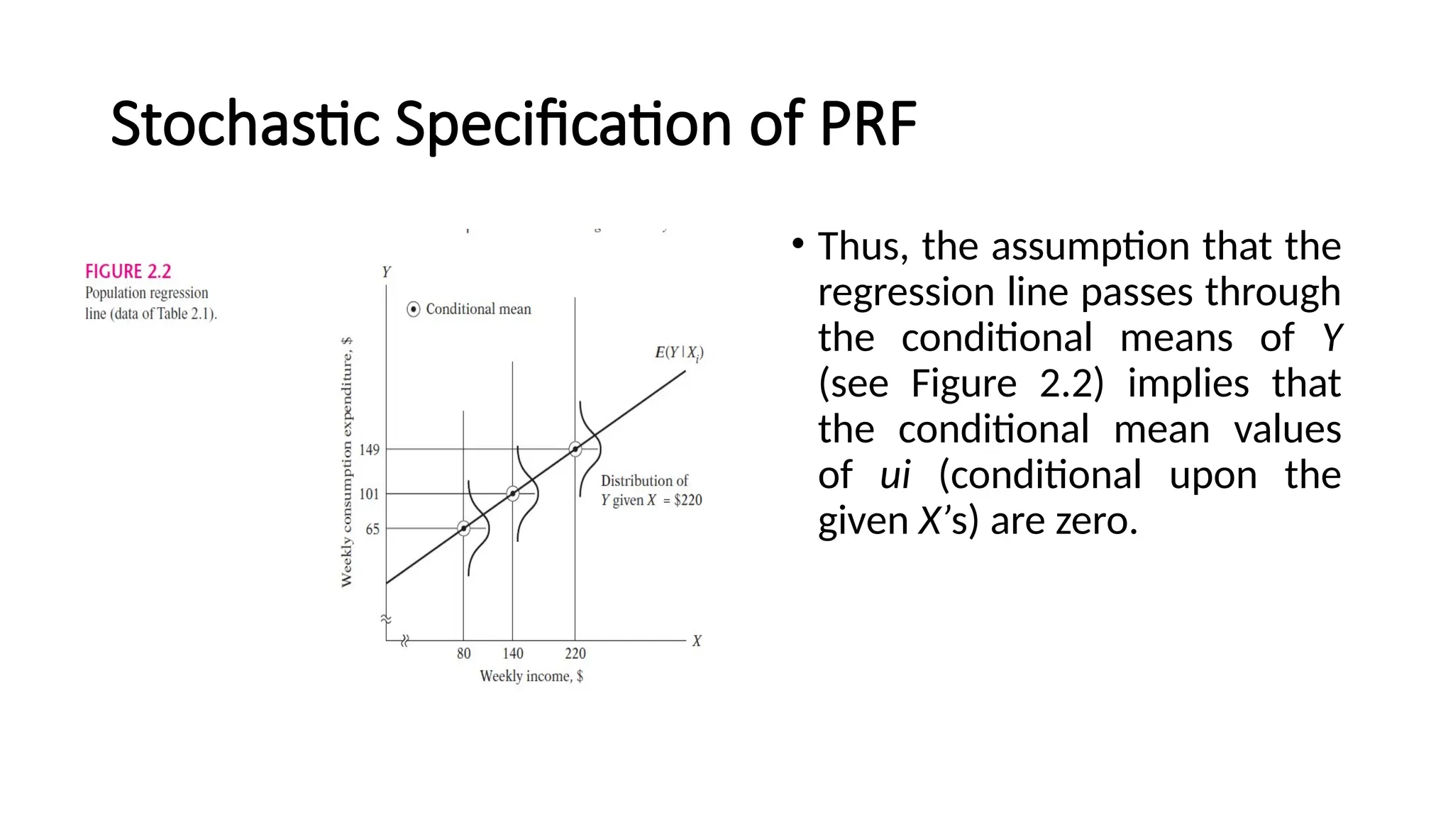
26. • Thus, the assumption that the
regression line passes through
the conditional means of Y
(see Figure 2.2) implies that
the conditional mean values
of ui (conditional upon the
given X’s) are zero.
Stochastic Specification of PRF

27. The Significance of the Stochastic Disturbance
Term
1. Vagueness of theory: The theory, if any, determining the behavior of
Y may be, and often is, incomplete.
• We might know for certain that weekly income X influences weekly
consumption expenditure Y, but we might be ignorant or unsure
about the other variables affecting Y.
• Therefore, may be used as a substitute for all the excluded or omitted
variables from the model.

28. 2. Unavailability of data: Even if we know what some of the excluded
variables are and therefore consider a multiple regression rather than a
simple regression, we may not have quantitative information about
these variables.
3. Core variables versus peripheral variables: But it is quite possible that
the joint influence of all or some of these variables may be so small.
• One hopes that their combined effect can be treated as a random
variable
The Significance of the Stochastic Disturbance
Term

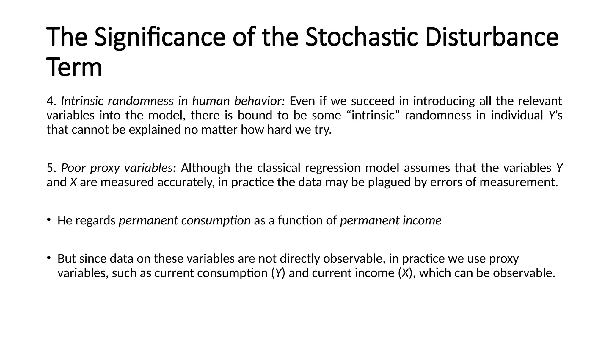
29. 4. Intrinsic randomness in human behavior: Even if we succeed in introducing all the relevant
variables into the model, there is bound to be some “intrinsic” randomness in individual Y’s
that cannot be explained no matter how hard we try.
5. Poor proxy variables: Although the classical regression model assumes that the variables Y
and X are measured accurately, in practice the data may be plagued by errors of measurement.
• He regards permanent consumption as a function of permanent income
• But since data on these variables are not directly observable, in practice we use proxy
variables, such as current consumption (Y) and current income (X), which can be observable.
The Significance of the Stochastic Disturbance
Term

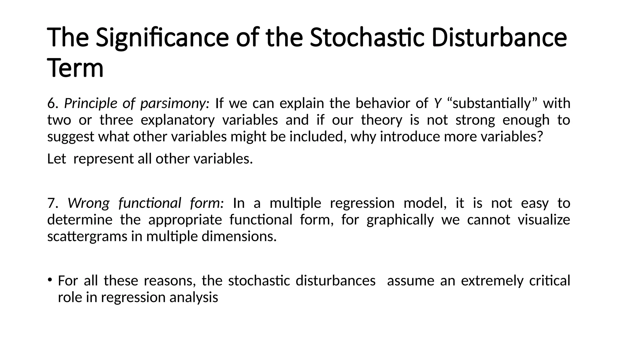
30. 6. Principle of parsimony: If we can explain the behavior of Y “substantially” with
two or three explanatory variables and if our theory is not strong enough to
suggest what other variables might be included, why introduce more variables?
Let represent all other variables.
7. Wrong functional form: In a multiple regression model, it is not easy to
determine the appropriate functional form, for graphically we cannot visualize
scattergrams in multiple dimensions.
• For all these reasons, the stochastic disturbances assume an extremely critical
role in regression analysis
The Significance of the Stochastic Disturbance
Term

31. The Sample Regression Function (SRF)
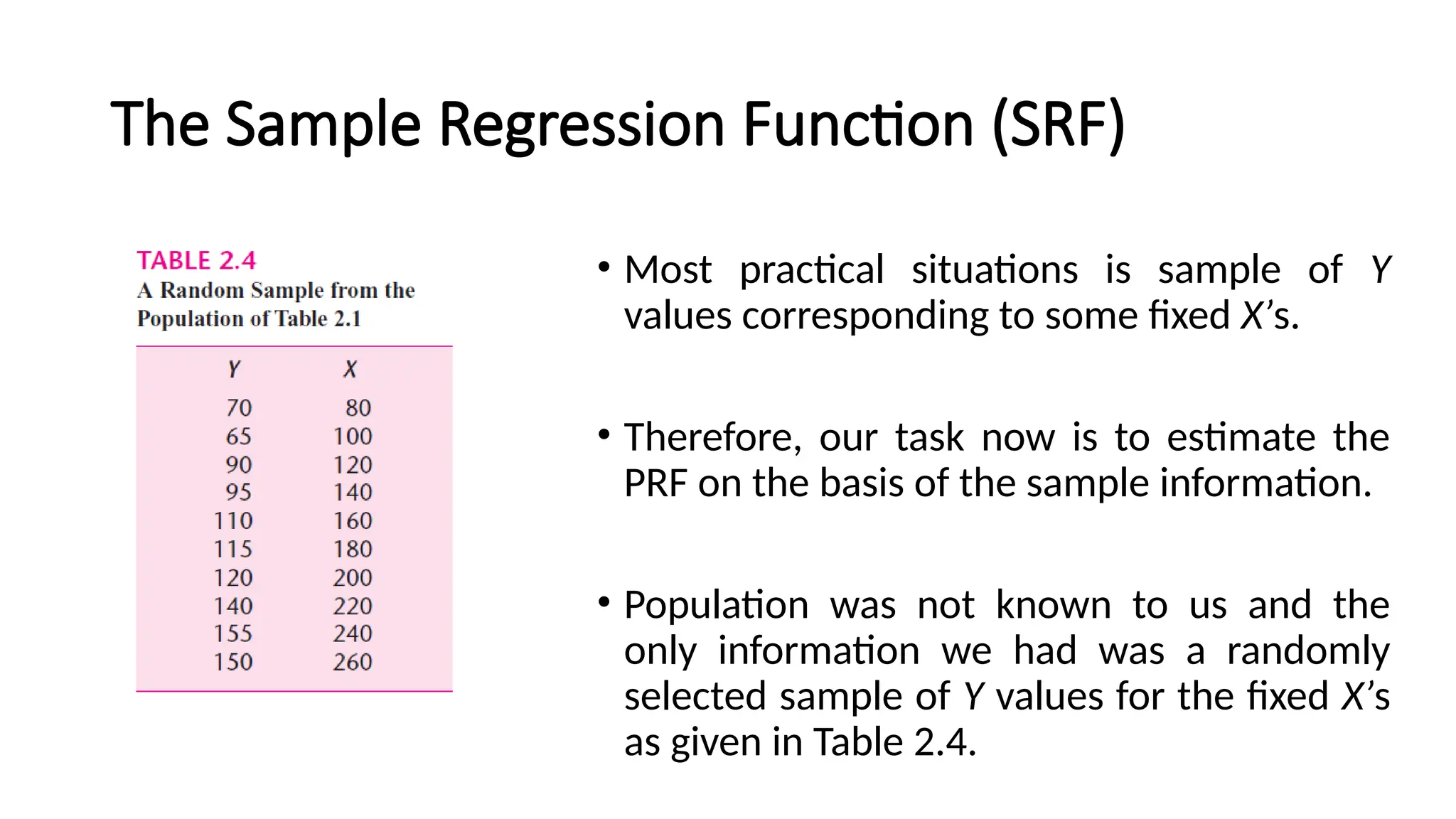
• Most practical situations is sample of Y
values corresponding to some fixed X’s.
• Therefore, our task now is to estimate the
PRF on the basis of the sample information.
• Population was not known to us and the
only information we had was a randomly
selected sample of Y values for the fixed X’s
as given in Table 2.4.

32. The Sample Regression Function (SRF)
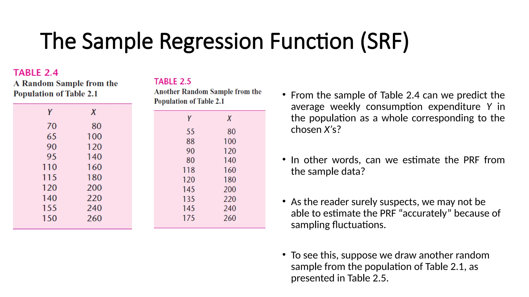
• From the sample of Table 2.4 can we predict the
average weekly consumption expenditure Y in
the population as a whole corresponding to the
chosen X’s?
• In other words, can we estimate the PRF from
the sample data?
• As the reader surely suspects, we may not be
able to estimate the PRF “accurately” because of
sampling fluctuations.
• To see this, suppose we draw another random
sample from the population of Table 2.1, as
presented in Table 2.5.

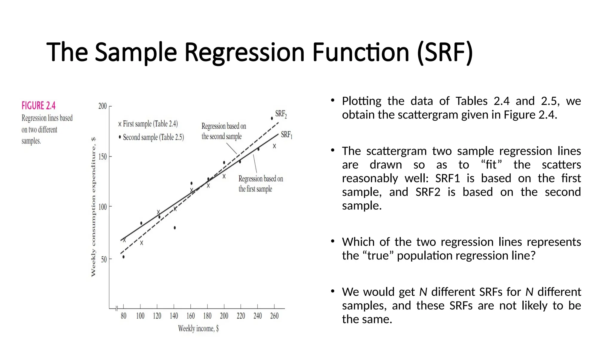
33. • Plotting the data of Tables 2.4 and 2.5, we
obtain the scattergram given in Figure 2.4.
• The scattergram two sample regression lines
are drawn so as to “fit” the scatters
reasonably well: SRF1 is based on the first
sample, and SRF2 is based on the second
sample.
• Which of the two regression lines represents
the “true” population regression line?
• We would get N different SRFs for N different
samples, and these SRFs are not likely to be
the same.
The Sample Regression Function (SRF)

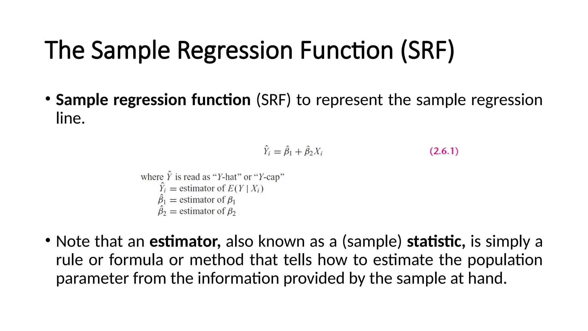
34. • Sample regression function (SRF) to represent the sample regression
line.
• Note that an estimator, also known as a (sample) statistic, is simply a
rule or formula or method that tells how to estimate the population
parameter from the information provided by the sample at hand.
The Sample Regression Function (SRF)

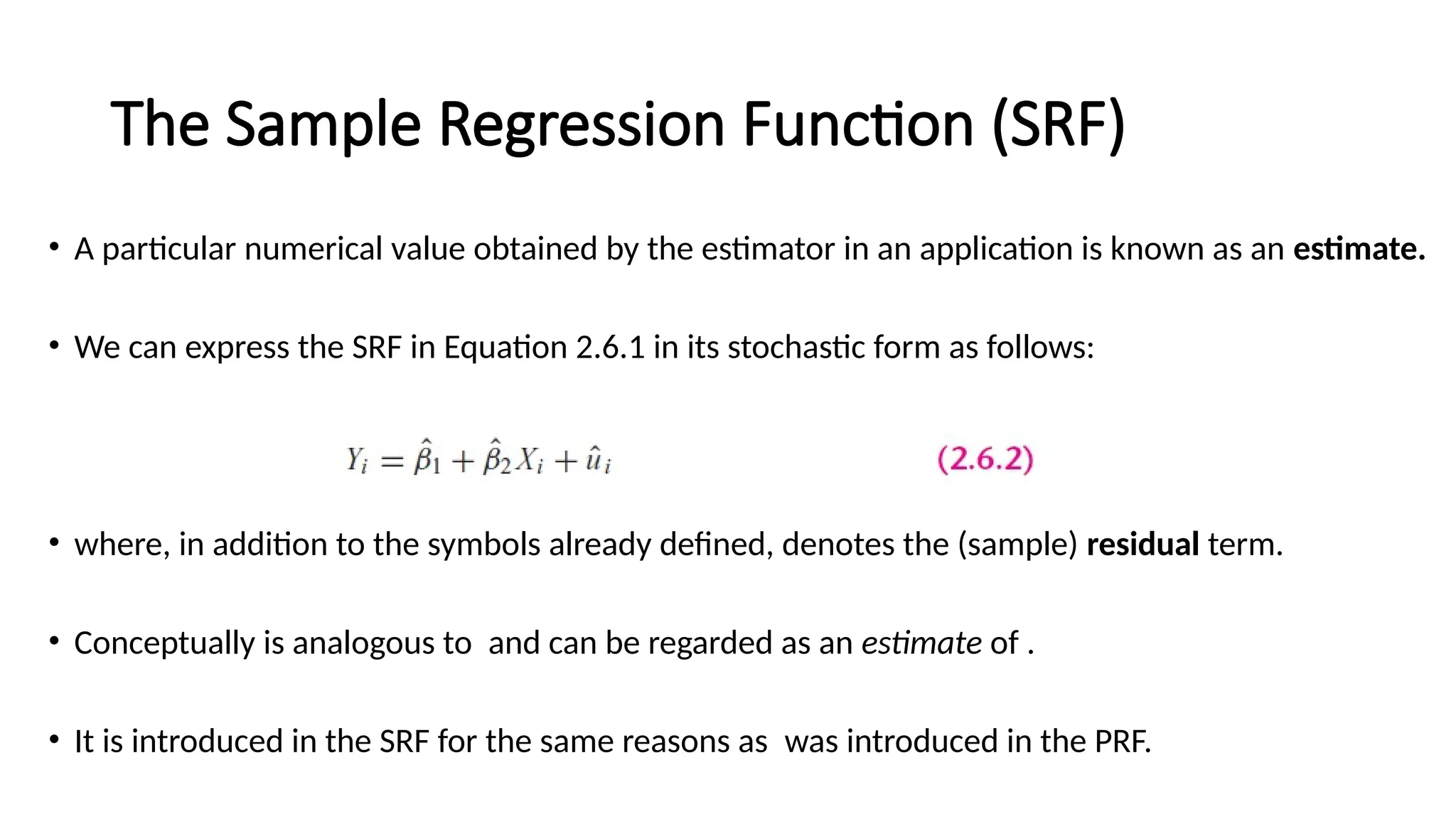
35. • A particular numerical value obtained by the estimator in an application is known as an estimate.
• We can express the SRF in Equation 2.6.1 in its stochastic form as follows:
• where, in addition to the symbols already defined, denotes the (sample) residual term.
• Conceptually is analogous to and can be regarded as an estimate of .
• It is introduced in the SRF for the same reasons as was introduced in the PRF.
The Sample Regression Function (SRF)

36. • For , we have one (sample)
observation, .
• In terms of the SRF, the
observed Yi can be expressed as
and in terms of the PRF, it can be
expressed as
The Sample Regression Function (SRF)

37. THANK YOU