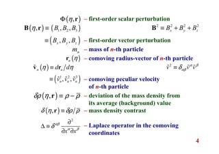
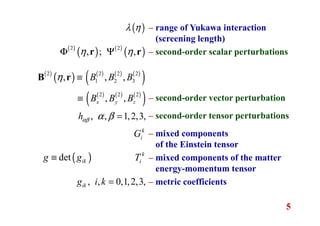
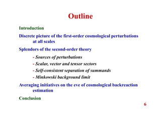
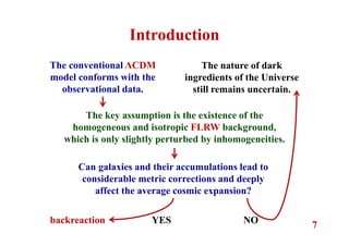
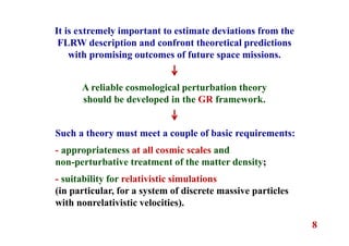
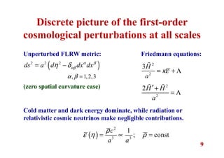
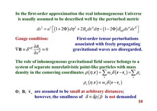
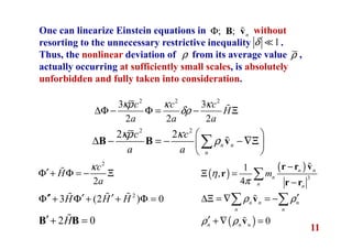
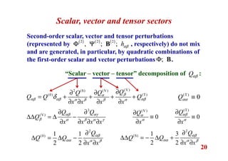
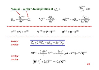
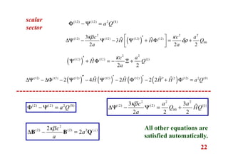
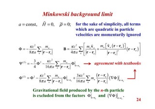
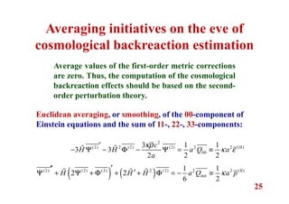
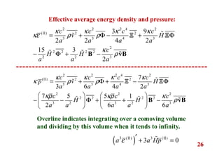
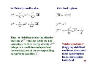
The document discusses second-order cosmological perturbations caused by point-like masses, building upon earlier works by Brilenkov and Eingorn. It highlights the need for a reliable cosmological perturbation theory within general relativity that accommodates all scales and does not impose limitations on mass density treatment. The study aims to understand the impact of inhomogeneous gravitational fields on cosmic expansion and metric corrections.

1. Ruslan Brilenkov 1, 2
Maxim Eingorn 3
1 University of Innsbruck, Institute for Astro- and Particle Physics,
Innsbruck, Austria
2 Università di Padova, Dipartimento di Fisica e Astronomia
‘G. Galilei’, Padova, Italy
3 North Carolina Central University, CREST and NASA Research
Centers, Durham, North Carolina, U.S.A.
Second-order Cosmological Perturbations
Engendered by Point-like Masses

2. 2
References
R. Brilenkov and M. Eingorn, Second-order cosmological perturbations
engendered by point-like masses, Astrophysical Journal 845, 153 (2017)
{ paper which this presentation is based on }
M. Eingorn, First-order cosmological perturbations
engendered by point-like masses, Astrophysical Journal 825, 84 (2016)
{ original paper on analytical perturbation theory covering all scales }
M. Eingorn, All-scale cosmological perturbations and screening of gravity
in inhomogeneous Universe
{ presentation based on the original paper }
M. Eingorn, Cosmological law of universal gravitation,
International Journal of Modern Physics D 26, 1750121 (2017)
{ essay on aspects of screening in the context of equations of motion }

3. 3
Notation
η – conformal time
– comoving coordinates
– scale factor
– speed of light
– Newtonian gravitational constant
– derivative with respect to
– energy density of nonrelativistic
pressureless matter (CDM + baryons)
– averaging
– cosmological constant (representing dark energy)
– mass density in the comoving coordinates
, 1,2,3,xα
α =
( )a η
( )H a aη ′≡ɶ
4
8 NG cκ π≡
NG
c
prime η
( ),ε η r
overline
Λ
( ),ρ η r

4. 4
– first-order scalar perturbation
– first-order vector perturbation
– mass of n-th particle
– comoving radius-vector of n-th particle
– comoving peculiar velocity
of n-th particle
– deviation of the mass density from
its average (background) value
– mass density contrast
– Laplace operator in the comoving
coordinates
( ),ηΦ r
( ) ( )
( )
1 2 3, , ,
, ,x y z
B B B
B B B
η ≡
≡
B r
nm
( )n ηr
( )
( )1 2 3
, ,
n n
n n n
d d
v v v
η η≡
≡
v rɶ
ɶ ɶ ɶ
( ),δρ η ρ ρ≡ −r
( ),δ η δρ ρ≡r
2
x x
αβ
α β
δ
∂
∆ ≡
∂ ∂
2 2 2 2
x y zB B B≡ + +B
2
v v vα β
αβδ≡ɶ ɶ ɶ

5. 5
– range of Yukawa interaction
(screening length)
– second-order scalar perturbations
– second-order vector perturbation
– second-order tensor perturbations
– mixed components
of the Einstein tensor
– mixed components of the matter
energy-momentum tensor
– metric coefficients
( )λ η
( )
( ) ( )
( )2 2
, ; ,η ηΦ Ψr r
( )
( ) ( ) ( ) ( )
( )
( ) ( ) ( )
( )
2 2 2 2
1 2 3
2 2 2
, , ,
, ,x y z
B B B
B B B
η ≡
≡
B r
, , 1,2,3,hαβ α β =
k
iG
k
iT( )det ikg g≡
, , 0,1,2,3,ikg i k =

6. 6
Outline
Introduction
Discrete picture of the first-order cosmological perturbations
at all scales
Splendors of the second-order theory
- Sources of perturbations
- Scalar, vector and tensor sectors
- Self-consistent separation of summands
- Minkowski background limit
Averaging initiatives on the eve of cosmological backreaction
estimation
Conclusion

7. 7
The conventional ΛCDM
model conforms with the
observational data.
The nature of dark
ingredients of the Universe
still remains uncertain.
Introduction
The key assumption is the existence of the
homogeneous and isotropic FLRW background,
which is only slightly perturbed by inhomogeneities.
Can galaxies and their accumulations lead to
considerable metric corrections and deeply
affect the average cosmic expansion?
backreaction YES NO

8. 8
It is extremely important to estimate deviations from the
FLRW description and confront theoretical predictions
with promising outcomes of future space missions.
A reliable cosmological perturbation theory
should be developed in the GR framework.
Such a theory must meet a couple of basic requirements:
- appropriateness at all cosmic scales and
non-perturbative treatment of the matter density;
- suitability for relativistic simulations
(in particular, for a system of discrete massive particles
with nonrelativistic velocities).

9. 9
Discrete picture of the first-order
cosmological perturbations at all scales
Unperturbed FLRW metric:
( )2 2 2
ds a d dx dxα β
αβη δ= −
, 1,2,3α β =
(zero spatial curvature case)
Friedmann equations:
2
2
3H
a
κε= + Λ
ɶ
2
2
2H H
a
′+
= Λ
ɶ ɶ
Cold matter and dark energy dominate, while radiation or
relativistic cosmic neutrinos make negligible contributions.
( )
2
3 3
1
; const
c
a a
ρ
ε η ρ= ∝ =

10. 10
In the first-order approximation the real inhomogeneous Universe
is usually assumed to be described well by the perturbed metric
( ) ( )2 2 2
1 2 2 1 2ds a d B dx d dx dxα α β
α αβη η δ = + Φ + − − Φ 
Gauge condition:
0
B
x
αβ α
β
δ
∂
∇ ≡ ≡
∂
B
First-order tensor perturbations
associated with freely propagating
gravitational waves are disregarded.
The role of inhomogeneous gravitational field source belongs to a
system of separate nonrelativistic point-like particles with mass
density in the comoving coordinates ( ) ( ), n n n
n n
mρ η δ ρ= − =∑ ∑r r r
( ) ( ),n n nmρ η δ≡ −r r r
; ; nΦ B vɶ are assumed to be small at arbitrary distances;
however, the smallness of is not demandedδ δρ ρ≡

11. 11
One can linearize Einstein equations in without
resorting to the unnecessary restrictive inequality .
Thus, the nonlinear deviation of from its average value ,
actually occurring at sufficiently small scales, is absolutely
unforbidden and fully taken into consideration.
; ; nΦ B vɶ
2 2 2
3 3
2 2 2
c c c
H
a a a
κρ κ κ
δρ∆Φ − Φ = − Ξɶ
2 2
2 2
n n
n
c c
a a
κρ κ
ρ
 
∆ − = − −∇Ξ 
 
∑B B vɶ
( )
( )
3
1
,
4
n n
n
n n
mη
π
−
Ξ =
−
∑
r r v
r
r r
ɶ
1δ ≪
ρρ
2
2
c
H
a
κ
′Φ + Φ = − Ξɶ
2
3 (2 ) 0H H H′′ ′ ′Φ + Φ + + Φ =ɶ ɶ ɶ
2 0H′+ =B Bɶ
n n n
n n
ρ ρ′∆Ξ = ∇ = −∑ ∑vɶ
( ) 0n n nρ ρ′ + ∇ =vɶ

12. 12
( )
( ) ( ) ( )
2
2
2
1
exp
3 8
1 1 exp3
8
n
n
n n
n n n n n
n n n
mc
q
a
m q qc
H
a q
κ
π
κ
π
Φ = − −
−
−  − + − + ⋅
−
∑
∑
r r
v r r
r r
ɶ
ɶ
( ) ( )
( )
( )
( ) ( )
2
2
2
2
3 2
3 2 3 4 exp 2 3 3
8
9 9 6 3 4 exp 2 3
n n n
n n
n n n
n n nn n n
n
nn
q q qmc
a q
q q qm
q
κ
π
 + + − −
= ⋅
 −

− + + −−   + − ⋅
−

∑
v
B
r r
v r r
r r
r r
ɶ
ɶ
Exact solutions of the Helmholtz equations:
( ), n
n
a
q η
λ
−
≡
r r
r
( ) ( )3 2 3 2
2 3a c aλ η κρ≡ ∝

13. 13
Sources of perturbations
Splendors of the second-order theory
( ) ( )
( )
2 2 2
2 (2) 2 (2) (2)
1 2 2 1 2
2 2 2
ds a d B dx d dx dx
a d B dx d h dx dx
α α β
α αβ
α α β
α αβ αβ
η η δ
η η δ
 = + Φ + − − Φ 
 + Φ + + Ψ + 
In the second-order approximation
(2)
(2)
0
B
x
αβ α
β
δ
∂
∇ ≡ ≡
∂
B
0
h
x
αγαβ
β
δ
∂
≡
∂
0hαβ
αβδ ≡
Gauge conditions:
k k k
i i iG Tκ δ= + ΛEinstein equations: , , 0,1,2,3i k =

14. 14
2
00 00
0
00 02
g v gc
T
g g g v g v v
γ
γ
α α β
α αβ
ρ +
= ⋅
− + +
ɶ
ɶ ɶ ɶ
2
00
00 02
g v gc
T
g g g v g v v
β
α αβ
α µ µ ν
µ µν
ρ +
= ⋅
− + +
ɶ
ɶ ɶ ɶ
( )2
0
00 02
v g v gc
T
g g g v g v v
α γ
β γβα
β µ µ ν
µ µν
ρ +
= ⋅
− + +
ɶ ɶ
ɶ ɶ ɶ
( )n n n n n
n n
v m v vα α α
ρ δ ρ≡ − =∑ ∑r rɶ ɶ ɶ
coincides
with in
the term
with factor
.
For instance,
nvα
ɶ
vα
ɶ
( )nδ −r r
Metric corrections which are generated by pure sources
and are assigned the first order: . Thus, for instance,
the term generates second-order metric corrections.
δρ
nvɶ ;Φ B
δρ∝ ⋅Φ

15. 15
( )
2
2 (2) 2 (2) (2)
2 2 2 2 2 2 2
2 2 2 2
(2)
003 3 3 3
3 2 6 6 2 6 6
3 3
H
H H H H
a a a a a a a
c c c c
Q
a a a a
κρ κ κρ κρ
δρ
   ′′+ ∆Φ − Φ − Φ + ∆Ψ − Φ − Ψ   
   
 
= + Λ + + Φ + Ψ + 
 
ɶ
ɶ ɶ ɶ ɶ
( )(2)(2)
(2)
2 2 2 2 2 2
2 2 2
(2)
03 3 3
1 2 2 1 2 2
2 2
B H B H
a a x a x a a x a x
c c c
B v B Q
a a a
β ββ β β β
β
β β β
κρ κ κρ
ρ
 ′∂ Ψ′∂Φ ∂Φ ∂Φ   ∆ + + + ∆ + +   ∂ ∂ ∂ ∂   
 
 
= − + + 
 
ɶ ɶ
ɶ
Einstein equations up to the second order
in metric corrections and their sources:
00-component:
0β-components:

16. 16
( )
( ) ( ) ( ) ( )
( )
2
2
2 2 2 2 2 2
2 (2) (2) (2) (2)
2 2 2 2
(2) 2 (2) 2 (2)
(2) (2) (2)
2 2 2 2 2 2 2 2
112
2 2 6 2 2 1
2
2 2 4 2
2
2 1 1 1 1 1
1
2
x x
x
x
B BH H
H H H H
a a a a a x a x
H H H H
a a a a
B
H B
a x a x a x a x a a
h
a
′′ ∂ ∂+  
′ ′ ′′− + Φ + Φ + Φ + + 
∂ ∂ 
 ′ ′ ′′′− + Φ + Φ + Ψ + Ψ

∂ ∂ ∂ Φ ∂ Ψ′+ + − + + ∆Φ − ∆Ψ 
∂ ∂ ∂ ∂ 
′′+
ɶ ɶ
ɶ ɶ ɶ ɶ
ɶ ɶ ɶ ɶ
ɶ
11 11 112 2
1 1
2
Hh h Q
a a
′+ − ∆ = Λ +ɶ
11-component (22- and 33-components are analogous):
( ) ( )
2 2 2 2
(2)(2) 2 (2) 2 (2)
(2) (2)
2 2 2 2 2 2
12 12 12 122 2 2
1 1 1 1
2 2
1 1 1 1 1 1
2 2
1 1 1
2 2
y yx x
yx
x y
B BB B
H H
a y a y a x a x
BB
H B H B
a y a y a x a x a x y a x y
h Hh h Q
a a a
′∂ ∂′ ∂ ∂
− + + + 
∂ ∂ ∂ ∂ 
 ∂∂ ∂ ∂ ∂ Φ ∂ Ψ′ ′− + + + − +  ∂ ∂ ∂ ∂ ∂ ∂ ∂ ∂ 
′′ ′+ + − ∆ =
ɶ ɶ
ɶ ɶ
ɶ
12-component (13- and 23-components are analogous):

17. 17
( )
( ) ( )
2 2 4 2 2
2 2 2 2
00 3 4 3 3 2
2
22 2
3 2 2 2 2
2
2
2 2 2 3
3 6 3 15
2 4 2
3 2 3 2
2
1 1 1
4 8 4
c c c c
Q v H H
a a a a a
c
H H
a a a a a
c
a a a a
κ κ κ κρ
ρ
κρ
κ
ρ
 
= − Ξ + ΞΦ − + Φ 
 
 
+ + − Φ∆Φ − ∇Φ + ∇Φ 
 
− ∆ + ∆ + ∇ ∇ −  
B B
B B B B B vB
ɶ ɶɶ
ɶ ɶ
ɶ
( )
( )
22 2 2
0 3 3 3 2 2
2 2 2
2 3 2 2
1 1
5 1 1
c c c
Q B B v B H
a a a a a x
Bc
H B
a x a x a x x a x x
β
β β β β β
γαγ αγ
γβ β β α α β
κ κρ κ
δρ ρ
κ
δ δ
∂
= + Φ + Φ − ∆Φ −
∂
∂ Φ ∂∂Φ ∂Φ ∂ Φ
+ + Ξ + −
∂ ∂ ∂ ∂ ∂ ∂
B
ɶɶ
ɶ
00 0 11 12, , ,Q Q Q Qβ
0
,
Q
Q
x
β
ααβ
∂
∂
? ?

18. 18
( )
( ) ( )
2 2 4 2 2
2 2 2 2 2 2
11 3 4 3 3 2 2
22
2
2 2 2 2 2 2 2
2 2
2
2 2 2 3 3
2
2 3
3 4 5 1
4
4 4 3 2 2 3
4
1 1 1
2 8 4
2
x
x
x x x x
x
c c c c
Q v H H H
a a a a a a
HB
a a x a a x a x a
c c
B B v B
a a a a a
B c
H
a x a
κ κ κ κρ
ρ
κ κ
ρ ρ
κ
 
= − − Ξ + ΞΦ + − Φ − 
 
∂ Φ ∂Φ ∂Φ 
− Φ∆Φ + Φ − ∇Φ + − − ∆ 
∂ ∂ ∂ 
+ ∆ + ∆ − ∇ ∇ − +  
∂
+ Φ + Ξ
∂
B
B B
B B B vB
ɶ ɶ ɶɶ
ɶ
ɶ ɶ
ɶ
2 2
2 2 2
2 22 2
2 2 2 2 2 2
1 1 1
2 2
1 1 1 1
y yx z z
y yz z
z y y z
B BB B B
x a z y a z a y
B BB B
B B B B
a y a z a y z a y z
∂ ∂   ∂ ∂ ∂
− + +   
∂ ∂ ∂ ∂ ∂  
∂ ∂∂ ∂
+ + − −
∂ ∂ ∂ ∂ ∂ ∂
( ) ( )
2
0 2 201 02 03
3 2 2
2 2 2
3 3 3
1 5
3
Q Q Q Q c
H H
x x y z a a a
c c c
H
a a a
β
β
κ
κ κ κ
ρ
∂  ∂ ∂ ∂
≡ + + = ∆ ΞΦ − + Φ 
∂ ∂ ∂ ∂  
− ∇Φ + ∇Φ∇Ξ + ∇Ξ
B
v B
ɶ ɶ
ɶɶ

19. 19
2 2 22 2
12 3 3 2 2 2 2 2 2
2 2 2
2 2 2 2 2
2
2 2 3 2
1 1 1
2 2 4 4 4
1 1 1 1 1
2 2 2 4 2
1 1 1
4 2
x x x
y x y x y y y
y y y yxz z
y z z
x xz z
x
B B Bc c
Q v B v v B B B
a a a z a y a x
B B B BBB B
B B B
a x y a x z a x y a z z a z x
B BB B c
H HB
a y x a y a y a y
κ κ
ρ ρ
κ
∂ ∂ ∂
= − − + −
∂ ∂ ∂
∂ ∂ ∂ ∂∂∂ ∂
− + − − +
∂ ∂ ∂ ∂ ∂ ∂ ∂ ∂ ∂ ∂
∂ ∂∂ ∂ ∂Φ
− + Φ + Ξ − +
∂ ∂ ∂ ∂ ∂
ɶ ɶ ɶ
ɶ ɶ
2
2 2
1 2
a y x a x y
∂Φ ∂Φ ∂ Φ
+ Φ
∂ ∂ ∂ ∂
+
( )
( ) ( )
2 2 4 2
2 2
11 22 33 3 4 3
2
22 2 2 2
3 2 2 2 2 2
2
2
2 2 2 3
3 9
4
12 15 3 8 7 2
5 5 3 2
4 8 4
c c c
Q Q Q Q v H
a a a
c
H H H
a a a a a a
c
a a a a
αα
κ κ κ
ρ
κρ
κ
ρ
≡ + + = − − Ξ + ΞΦ
 
+ − Φ − − Φ∆Φ − ∇Φ − ∇Φ 
 
− ∆ + ∆ − ∇ ∇ −  
B B
B B B B B vB
ɶɶ
ɶ ɶ ɶ
ɶ
exactly the same terms with replacement x y↔

20. 20
Scalar, vector and tensor sectors
Second-order scalar, vector and tensor perturbations
(represented by , respectively) do not mix
and are generated, in particular, by quadratic combinations of
the first-order scalar and vector perturbations .;Φ B
( ) ( ) ( )2 2 2
, ; ; hαβΦ Ψ B
“Scalar – vector – tensor” decomposition of :Qαβ
(V)(V)2 (S)
(0) (T)
QQQ
Q Q Q
x x x x
βα
αβ αβ αβα β β α
δ
∂∂∂
= + + + +
∂ ∂ ∂ ∂
(V)
0
Q
x
α
α
∂
≡
∂
(T)
0
Q
x
αβ
α
∂
≡
∂
(T)
0Qαα ≡
2
(0) 1 1
2 2
Q
Q Q
x x
αβ
αα α β
∂
∆ = ∆ −
∂ ∂
2
(S) 1 3
2 2
Q
Q Q
x x
αβ
αα α β
∂
∆∆ = − ∆ +
∂ ∂
3
(V)
Q Q
Q
x x x x
αβ αγ
β α β α γ
∂ ∂
∆∆ = ∆ −
∂ ∂ ∂ ∂

21. 21
“Scalar – vector” decomposition of :0Q α
( )
( )
0
Q
Q Q
x
α αα
⊥∂
= +
∂
( )
0
Q
x
α
α
⊥
∂
≡
∂
( ) 0Q
Q
x
α
α
∂
∆ =
∂
2
0( )
0
Q
Q Q
x x
β
α α α β
⊥
∂
∆ = ∆ −
∂ ∂
(12) (2)
Φ ≡ Φ + Φ (12) (2)
Ψ ≡ Φ + Ψ (12) (2)
≡ +B B B
2 (T)
2 2h Hh h a Qαβ αβ αβ αβ
′′ ′+ − ∆ =ɶ
( )
2 2
(12) (12) 2 ( )2 2
2
c c
a
a a
κρ κ
ρ ⊥
∆ − = − − ∇Ξ +B B v Qɶ
( )(12) (12) 2 (V)
2 2H a′ + = −B B Qɶ
tensor
sector
vector
sector

22. 22
scalar
sector
(12) (12) 2 (S)
a QΦ − Ψ =
( )
2 2 2
(12) (12) (12) (12)
00
3
3
2 2 2
c c a
H H Q
a a
κρ κ
δρ
 ′∆Ψ − Ψ − Ψ + Φ = +  
ɶ ɶ
( )
2 2
(12) (12) ( )
2 2
c a
H Q
a
κ′Ψ + Φ = − Ξ +ɶ
( ) ( ) ( ) ( )(12) (12) (12) (12) (12) 2 (12) 2 (0)
2 4 2 2 2H H H H a Q′′ ′ ′ ′∆Ψ − ∆Φ − Ψ − Ψ − Φ − + Φ =ɶ ɶ ɶ ɶ
2
(2) (2) 2 ( )2
2
c
a
a
κρ ⊥
∆ − =B B Q
(2) (2) 2 (S)
a QΦ − Ψ =
2 2 2
(2) (2) ( )
00
3 3
2 2 2
c a a
Q HQ
a
κρ
∆Ψ − Ψ = + ɶ
All other equations are
satisfied automatically.

23. 23
Self-consistent separation of summands
Is the undertaken separation of the first- and second-order terms
well-grounded and self-consistent? In other words, are the orders
correctly and logically assigned to different summands?
The answer is yes: at any cosmological scale for each summand in
the equations for the second-order metric corrections there exists
a much larger counterpart in the corresponding equations for the
first-order metric corrections.
Therefore, in particular, the situation when magnitudes of
and are comparable is really improbable. Quite the contrary,
the inequality may be expected to occur everywhere,
as it certainly should be in the framework of the self-consistent
perturbation theory.
( )2
Φ
Φ
( )2
Φ Φ≪

24. 24
Minkowski background limit
const, 0, 0;a H ρ= = =ɶ for the sake of simplicity, all terms
which are quadratic in particle
velocities are momentarily ignored
2
8
n
n n
mc
a
κ
π
Φ = −
−
∑ r r
( )
( )
2
3
4
n n nn n
n
n n n
mmc
a
κ
π
 −  = + − 
− −  
∑
v r rv
B r r
r r r r
ɶɶ
2
(2) 23
4 16 n
n
n n
mc
a
κ
π =
Ψ = − Φ − Φ
−
∑ r r
r r
( )
( )
2 2
(2) 2 3
8 16n n
nn
n
n nn n
mc c
m
a a
κ κ
π π= =
−
Φ = Φ − Φ + ∇Φ
− −
∑ ∑r r r r
r r
r r r r
Gravitational field produced by the n-th particle
is excluded from the factors and .n=
Φ r r
( ) n=
∇Φ r r
agreement with textbooks

25. 25
Averaging initiatives on the eve of
cosmological backreaction estimation
Average values of the first-order metric corrections
are zero. Thus, the computation of the cosmological
backreaction effects should be based on the second-
order perturbation theory.
Euclidean averaging, or smoothing, of the 00-component of
Einstein equations and the sum of 11-, 22-, 33-components:
2
(2) 2 (2) (2) 2 2 (II)
00
3 1 1
3 3
2 2 2
c
H H a Q a
a
κρ
κ ε
′
− Ψ − Φ − Ψ = ≡ɶ ɶ
( ) ( )(2) (2) (2) 2 (2) 2 2 (II)1 1
2 2
6 2
H H H a Q a pαα κ
′′′
′Ψ + Ψ + Φ + + Φ = − ≡ɶ ɶ ɶ

26. 26
2 2 2 4 2
(II) 2 2
3 3 4 3
2
2 2 2 2
2 2 3
3 9
2 2 4 2
15 3
2
c c c c
v H
a a a a
c
H H
a a a
κ κ κ κ
κε ρ ρ
κ
ρ
= + Φ − Ξ + ΞΦ
− Φ + −B vB
ɶɶ
ɶ ɶ ɶ
2 2 2 4 2
(II) 2 2
3 3 4 3
2 2 2
2 2 2 2
3 2 3 2 3
7
3 6 4 2
7 5 5 1
2 6 6
c c c c
p v H
a a a a
c c c
H H
a a a a a
κ κ κ κ
κ ρ ρ
κρ κρ κ
ρ
= + Φ + Ξ − ΞΦ
   
− − Φ + + −   
   
B vB
ɶɶ
ɶ ɶ ɶ
Effective average energy density and pressure:
Overline indicates integrating over a comoving volume
and dividing by this volume when it tends to infinity.
( )3 (II) 3 (II)
3 0a a Hpε ′ + =ɶ

27. 27
Sufficiently small scales:
2 2
(II) 2
3 3
2 2
c c
v
a a
ε ρ ρ= + Φɶ
2 2
(II) 2
3 3
3 6
c c
p v
a a
ρ ρ= + Φɶ
Virialized regions:
Thus, at virialized scales the effective
pressure vanishes while the non-
vanishing effective energy density
brings to a small time-independent
renormalization of the corresponding
background quantity .
“Stable clustering”
(implying virialized
nonlinear structures)
razes backreaction
from cosmological
battlefield.
2
2 vρ ρΦ = − ɶ
(II)
0p →
2
(II) 2
3 3
1
2
c
v
a a
ε ρ→ − ∝ɶ
(II)
p
(II)
ε
ε

28. 28
- launch of a new generation of cosmological N-body simulations
based on the developed formalism;
- use of outputs of these simulations for the estimation of
the effective average energy density and pressure , and
subsequent comparison with the background quantity ;
- estimation of , and subsequent comparison
with , respectively.
Feasible plan to estimate cosmological backreaction:
(II)
ε
(II)
p
ε
( ) ( ) ( )2 2 2
, ;Φ Ψ B
;Φ B
at any moment during the matter-
dominated or Λ-dominated stages of the Universe
evolution backreaction significance; inappropriateness
of FLRW metric and Friedmann equations,
with inevitable grave consequences…
(II) (II)
, ~pε εIf

29. 29
The proposed plan exploits Yukawa gravity resulting from GR
and therefore possesses a definite advantage over the generally
accepted simulations exploiting Newtonian gravity, which does
not represent the weak field limit of GR.
Yukawa screening of interparticle attraction may be treated
as a relativistic effect. This is especially important in view of
the fact that backreaction significance is inseparably linked
with non-Newtonian gravitational physics.
In the framework of the so-called Newtonian cosmology,
as opposed to GR, the backreaction effects are reduced
to boundary terms vanishing in the case of the standard
periodic boundary conditions.
Averaged expansion rate? Effective equation of state?
Kinematical and dynamical backreactions?

30. 30
-- Equations for second-order scalar, vector, tensor cosmological
perturbations are derived. These equations are suitable at all
spatial scales and permit of nonlinear density contrasts;
- all Einstein equations are satisfied within the adopted accuracy
along with the gauge conditions;
- self-consistency of order assignments and related expectation
that the first-order metric corrections dominate over the second-
order ones everywhere are confirmed;
- in the Minkowski background limit the linkage with textbook
material is established;
---- highway to investigate the cosmological backreaction effects
beyond Newtonian gravitational physics is outlined.
Conclusion