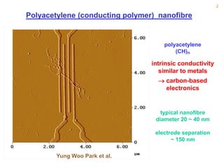
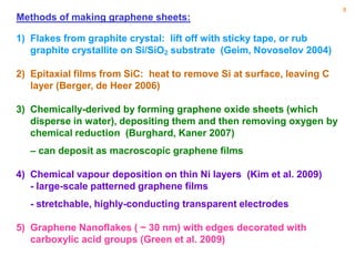
17 October 2011
             NZ Institute of Physics Conference


                      Alan B. Kaiser
          Shrividya Ravi and Chris Bumby *
MacDiarmid Institute for Advanced Materials and Nanotechnology,
                Victoria University of Wellington
         * Now at Industrial Research Ltd, Gracefield


                                VICTORIA UNIVERSITY OF WELLINGTON
                                 Te Whare Wānanga o te Ūpoko o te Ika a Māui
2

Polyacetylene (conducting polymer) nanofibre


                                     polyacetylene
                                         (CH)n

                                 intrinsic conductivity
                                    similar to metals
                                    carbon-based
                                     electronics


                                    typical nanofibre
                                  diameter 20 ~ 40 nm

                                  electrode separation
                                        ~ 150 nm

        Yung Woo Park et al.
3

  Nobel prize for Physics 2010


               Andre Geim and Kostya Novoselov
  Awarded 2010 Nobel Prize for Physics for their ground- breaking
  experiments on the two-dimensional material graphene


- Demonstrated novel physics of electrons in graphene owing to
   unusual band structure around Fermi level.
4
Bulk graphite


                               loosely bound layers
                               of carbon atoms


Graphite flakes in pencil marks:


Including flakes only one atom
    thick!
Discovered by Andre Geim and
    his group, 2004
5
Resistance per square                 charge neutrality point
of graphene:


                     Resistance
                        (kW)
                                                                 electrons
        holes                                                    conduct
        conduct


                                  Gate voltage Vg shifts Fermi
                                     energy up (or down)

 Mobility can extremely high - up to 120,000 cm2/Vs at 240 K
 in suspended graphene
 (Andrei et al. 2008, Bolotin, Kim et al. 2008, Geim, Novoselov et al. 2008)

 - higher than any semiconductor (mean free path up to 1 mm)
6
Resistance of graphene flake
Viera Skákalová, Max Planck Institute, Stuttgart


                      charge neutrality point

          5


          4
                 before T-cycle
                 after T-cycle
 R (kW)


          3

                                                            Mesoscopic “Universal
          2                                                 Conductance
                                                            Fluctuations” very
          1                                                 persistent in graphene
                                                            - up to > 50 K
          -20   -15    -10   -5   0   5      10   15   20
                          Gate Voltage (V)
7
            Graphene: temperature dependence of resistance
                                                   Skakalova, Kaiser et al. Phys. Rev. B (2009)
                  1.4
                                                                         R(T) above 50K
                                                                         consistent with
                  1.2                                                    scattering by
                            low temperature
Resistance (kW)


                                                                         acoustic and high-
                            anomaly                                      energy phonons
                            - monotonic but                 high
                  1.0       can be up or down                            (as shown by Chen
                                                            energy       et al., Morosov et al.
                                                            phonons
                              fluctuations                               2008)

                  0.8                                              acoustic phonons

                            residual resistance

                  0.6
                        0       50     100        150    200      250
                                       Temperature (K)
8
Methods of making graphene sheets:

1) Flakes from graphite crystal: lift off with sticky tape, or rub
   graphite crystallite on Si/SiO2 substrate (Geim, Novoselov 2004)

2) Epitaxial films from SiC: heat to remove Si at surface, leaving C
   layer (Berger, de Heer 2006)

3) Chemically-derived by forming graphene oxide sheets (which
   disperse in water), depositing them and then removing oxygen by
   chemical reduction (Burghard, Kaner 2007)
   – can deposit as macroscopic graphene films

4) Chemical vapour deposition on thin Ni layers (Kim et al. 2009)
   - large-scale patterned graphene films
   - stretchable, highly-conducting transparent electrodes

5) Graphene Nanoflakes ( ~ 30 nm) with edges decorated with
   carboxylic acid groups (Green et al. 2009)
9
                 Reduced graphene oxide
Cristina Gómez-Navarro, Marko Burghard et al., Max Planck Institute, Stuttgart


 STM image:


                                   only parts of sample are oxidized
                                   in separation of graphene oxide
                                   sheets
                                   - remain disordered after oxygen
                                   removed by reduction

                                  well-ordered crystalline regions in
                                  regions not oxidized
10
 Conductance of reduced graphene oxide:
                                                                            Kaiser, Gómez-Navarro, Burghard et al., Nano Lett. (2009)
  2D variable-range hopping at high T                                                                                        -12

                                                                                                                                                              Vds            = 0.5 V
  for different gate voltages                                                                                                -14                            Vds= 0.5 V             (b)
(a)
                                                                                                                             -16
                        -12

                                                        Vds 0.1V0.1 V (c)
                                                        Vds= =


                                                                                                              ) (A)
                                                                                                                             -18
                        -14


                                                                                                       ln( I ln I (A)
                                                                                                                             -20
                        -16

                                                                                                                             -22
                        -18
      ln( I )ln I (A)
                  (A)


                                                                                                                             -24
                        -20                                                    Vg=-20V
                                                                               Vg=-15V
                                                                               Vg=-10V                                       -26
                        -22
                                                                               Vg=-5V                                        -12
                                                                                                                                0.1      0.2    0.3   0.4
                        -24
                                                                               Vg=0
                                                                               Vg=10V
                                                                                                                                                              V 0.6 2.0 V (a) 0.9
                                                                                                                                                              0.5
                                                                                                                                                                  = 0.7 0.8
                                                                                                                                                            Vds= 2 V
                                                                                                                                                                 ds
                                                                                                                                                               -1/3


                                                                                                         ln( I ln)I (A)(A)
                                                                                                                             -14                              T
                                                                               Vg=20V
                        -26
                                                                                                                             -16

                              0.1   0.2   0.3   0.4           0.5     0.6    0.7   0.8   0.9
                                                      1/3         -1/3                                                     -18
                                                 T(K
                                          1I T 1/3) (K-1/3)                                                                        0.1   0.2    0.3   0.4       0.5          0.6   0.7   0.8   0.9

                                                                                                                                               1I T 1/3) (K (K-1/3)
                                                                                                                                                             -1/3     -1/3
                                                                                                                                                      T      )


                               B 
             G(T )  G1 exp   1/ 3   G0                                                    temperature-independent conductance
                             T                                                               at low T, higher electric field
11
Conclusions on conduction mechanisms in reduced graphene
oxide:

 Conduction is highly heterogeneous:
 1) relatively high metallic conductivity in the crystalline regions
    with delocalized carrier density showing the usual
    dependence on gate voltage;
 2) thermally-driven variable-range hopping in disordered barrier
    regions that dominates the resistance above 40 K;
 3) purely field-driven T-independent tunnelling conduction at
    larger fields and low temperature: tunnelling between
    localized states in barrier regions, and through barrier regions
    at their thinnest points between delocalized states in metallic
    regions. The lowest barrier energies are inferred to be of
    order of 40 meV.


    These oxide-related barriers, if made in a controlled fashion,
    could define conducting channels on graphene sheets.
12

Applications of graphene:

1) Conducting composites with filling factors < 1%

2) Highly stretchable (up to 20% - more than any other crystal)

3) As membranes: gases cannot pass through monolayer
   graphene film

4) Support for samples in Transmission Electron Microscope

5) Ultra-sensitive chemical sensors (single molecules)

6) Nano-electro-mechanical systems (NEMS): light, stiff and strong

7) Graphene powder: Field emission


          (Geim and Novoselov, Nature Mater. 2007; Geim, Science 2009)
13

Towards Carbon-based Electronics:

1) Graphene with ballistic conduction at 300 K as very fast field-
   effect transistor (FET) (Avouris et al.)

2) Graphene nanoribbon transistors with band gap

3) Transistor circuitry could be created in a graphene sheet:
molecular electronics
but with top-down               gate
approach:


                                                                drain

            source
14
          Conduction in thick and thin SWCNT networks

  Measurements by Viera Skákalová, Max-Planck-Institut, Stuttgart


   thick network                                         Fluctuation-assisted
  (SWNT paper)                                           tunnelling between
approx 50 mm thick:                        1 mm
                                                         metallic regions


                                                         Variable-range
     thin network:                                       hopping between
                                                         localized states
                                             2 mm


        AFM trace:                                 50 nm 
                                                   50 nm
15

                               Transparency of thin SWCNT networks

                                                  Thick free-standing
                                                   SWCNT network
          Conductance per squareS(S)
            Square Conductance( )           1
                                       10       Buckypaper
                                            0
                                       10
                                                                         SWCNT networks
                                        -1
                                       10                                 become thinner
                                        -2
                                       10        Net 4
                                                         Net 3
                                        -3                       Net 2
                                       10
                                        Net 1
                   0    20   40    60    80 100
                         Transmittance (%)
Net 4 made with 4 return                    Net 1 made with 1 return
   air-brush strokes                            air-brush stroke

                                                 Measurements by Viera Skákalová, MPI Stuttgart
16
Thin transparent single-wall carbon nanotube films:
Shrividya Ravi and Dr Chris Bumby (Victoria University of Wellington)


     drop casting with SWCNTs
             
     in solvent on square glass
                     cover slip:


      very thin SWCNT film with
                 metal contacts


                     thicker film
17

Rolled-up Graphene: Single-Wall Carbon Nanotube thin networks
Enhancement of transmittance and conductance of
by removal of volatile solvent (butylamine):


                    annealed


         unannealed
                         Butylamine removed


             S. Ravi, A.B. Kaiser and C.L. Bumby, Chem. Phys Lett. (2010)
18
Conductance of single-wall carbon nanotube network (log scale)


                    variable-range hopping conduction


                                                  found „metallic‟
                                                   behaviour below 3 K
                    1/T1/4
   A few percolating metallic paths with thin tunnelling barriers -
   some similarity to chemically-derived graphene !


              S. Ravi, A.B. Kaiser and C.L. Bumby, Chem. Phys Lett. (2010)

15.30 o5 a kaiser

  • 1.
    17 October 2011 NZ Institute of Physics Conference Alan B. Kaiser Shrividya Ravi and Chris Bumby * MacDiarmid Institute for Advanced Materials and Nanotechnology, Victoria University of Wellington * Now at Industrial Research Ltd, Gracefield VICTORIA UNIVERSITY OF WELLINGTON Te Whare Wānanga o te Ūpoko o te Ika a Māui
  • 2.
    2 Polyacetylene (conducting polymer)nanofibre polyacetylene (CH)n intrinsic conductivity similar to metals  carbon-based electronics typical nanofibre diameter 20 ~ 40 nm electrode separation ~ 150 nm Yung Woo Park et al.
  • 3.
    3 Nobelprize for Physics 2010 Andre Geim and Kostya Novoselov Awarded 2010 Nobel Prize for Physics for their ground- breaking experiments on the two-dimensional material graphene - Demonstrated novel physics of electrons in graphene owing to unusual band structure around Fermi level.
  • 4.
    4 Bulk graphite loosely bound layers of carbon atoms Graphite flakes in pencil marks: Including flakes only one atom thick! Discovered by Andre Geim and his group, 2004
  • 5.
    5 Resistance per square charge neutrality point of graphene: Resistance (kW) electrons holes conduct conduct Gate voltage Vg shifts Fermi energy up (or down) Mobility can extremely high - up to 120,000 cm2/Vs at 240 K in suspended graphene (Andrei et al. 2008, Bolotin, Kim et al. 2008, Geim, Novoselov et al. 2008) - higher than any semiconductor (mean free path up to 1 mm)
  • 6.
    6 Resistance of grapheneflake Viera Skákalová, Max Planck Institute, Stuttgart charge neutrality point 5 4 before T-cycle after T-cycle R (kW) 3 Mesoscopic “Universal 2 Conductance Fluctuations” very 1 persistent in graphene - up to > 50 K -20 -15 -10 -5 0 5 10 15 20 Gate Voltage (V)
  • 7.
    7 Graphene: temperature dependence of resistance Skakalova, Kaiser et al. Phys. Rev. B (2009) 1.4 R(T) above 50K consistent with 1.2 scattering by low temperature Resistance (kW) acoustic and high- anomaly energy phonons - monotonic but high 1.0 can be up or down (as shown by Chen energy et al., Morosov et al. phonons fluctuations 2008) 0.8 acoustic phonons residual resistance 0.6 0 50 100 150 200 250 Temperature (K)
  • 8.
    8 Methods of makinggraphene sheets: 1) Flakes from graphite crystal: lift off with sticky tape, or rub graphite crystallite on Si/SiO2 substrate (Geim, Novoselov 2004) 2) Epitaxial films from SiC: heat to remove Si at surface, leaving C layer (Berger, de Heer 2006) 3) Chemically-derived by forming graphene oxide sheets (which disperse in water), depositing them and then removing oxygen by chemical reduction (Burghard, Kaner 2007) – can deposit as macroscopic graphene films 4) Chemical vapour deposition on thin Ni layers (Kim et al. 2009) - large-scale patterned graphene films - stretchable, highly-conducting transparent electrodes 5) Graphene Nanoflakes ( ~ 30 nm) with edges decorated with carboxylic acid groups (Green et al. 2009)
  • 9.
    9 Reduced graphene oxide Cristina Gómez-Navarro, Marko Burghard et al., Max Planck Institute, Stuttgart STM image: only parts of sample are oxidized in separation of graphene oxide sheets - remain disordered after oxygen removed by reduction well-ordered crystalline regions in regions not oxidized
  • 10.
    10 Conductance ofreduced graphene oxide: Kaiser, Gómez-Navarro, Burghard et al., Nano Lett. (2009) 2D variable-range hopping at high T -12 Vds = 0.5 V for different gate voltages -14 Vds= 0.5 V (b) (a) -16 -12 Vds 0.1V0.1 V (c) Vds= = ) (A) -18 -14 ln( I ln I (A) -20 -16 -22 -18 ln( I )ln I (A) (A) -24 -20 Vg=-20V Vg=-15V Vg=-10V -26 -22 Vg=-5V -12 0.1 0.2 0.3 0.4 -24 Vg=0 Vg=10V V 0.6 2.0 V (a) 0.9 0.5 = 0.7 0.8 Vds= 2 V ds -1/3 ln( I ln)I (A)(A) -14 T Vg=20V -26 -16 0.1 0.2 0.3 0.4 0.5 0.6 0.7 0.8 0.9 1/3 -1/3 -18 T(K 1I T 1/3) (K-1/3) 0.1 0.2 0.3 0.4 0.5 0.6 0.7 0.8 0.9 1I T 1/3) (K (K-1/3) -1/3 -1/3 T )  B  G(T )  G1 exp   1/ 3   G0 temperature-independent conductance  T  at low T, higher electric field
  • 11.
    11 Conclusions on conductionmechanisms in reduced graphene oxide: Conduction is highly heterogeneous: 1) relatively high metallic conductivity in the crystalline regions with delocalized carrier density showing the usual dependence on gate voltage; 2) thermally-driven variable-range hopping in disordered barrier regions that dominates the resistance above 40 K; 3) purely field-driven T-independent tunnelling conduction at larger fields and low temperature: tunnelling between localized states in barrier regions, and through barrier regions at their thinnest points between delocalized states in metallic regions. The lowest barrier energies are inferred to be of order of 40 meV. These oxide-related barriers, if made in a controlled fashion, could define conducting channels on graphene sheets.
  • 12.
    12 Applications of graphene: 1)Conducting composites with filling factors < 1% 2) Highly stretchable (up to 20% - more than any other crystal) 3) As membranes: gases cannot pass through monolayer graphene film 4) Support for samples in Transmission Electron Microscope 5) Ultra-sensitive chemical sensors (single molecules) 6) Nano-electro-mechanical systems (NEMS): light, stiff and strong 7) Graphene powder: Field emission (Geim and Novoselov, Nature Mater. 2007; Geim, Science 2009)
  • 13.
    13 Towards Carbon-based Electronics: 1)Graphene with ballistic conduction at 300 K as very fast field- effect transistor (FET) (Avouris et al.) 2) Graphene nanoribbon transistors with band gap 3) Transistor circuitry could be created in a graphene sheet: molecular electronics but with top-down gate approach: drain source
  • 14.
    14 Conduction in thick and thin SWCNT networks Measurements by Viera Skákalová, Max-Planck-Institut, Stuttgart thick network Fluctuation-assisted (SWNT paper) tunnelling between approx 50 mm thick: 1 mm metallic regions Variable-range thin network: hopping between localized states 2 mm AFM trace: 50 nm  50 nm
  • 15.
    15 Transparency of thin SWCNT networks Thick free-standing SWCNT network Conductance per squareS(S) Square Conductance( ) 1 10 Buckypaper 0 10 SWCNT networks -1 10 become thinner -2 10 Net 4 Net 3 -3 Net 2 10 Net 1 0 20 40 60 80 100 Transmittance (%) Net 4 made with 4 return Net 1 made with 1 return air-brush strokes air-brush stroke Measurements by Viera Skákalová, MPI Stuttgart
  • 16.
    16 Thin transparent single-wallcarbon nanotube films: Shrividya Ravi and Dr Chris Bumby (Victoria University of Wellington) drop casting with SWCNTs  in solvent on square glass cover slip: very thin SWCNT film with metal contacts thicker film
  • 17.
    17 Rolled-up Graphene: Single-WallCarbon Nanotube thin networks Enhancement of transmittance and conductance of by removal of volatile solvent (butylamine): annealed unannealed Butylamine removed S. Ravi, A.B. Kaiser and C.L. Bumby, Chem. Phys Lett. (2010)
  • 18.
    18 Conductance of single-wallcarbon nanotube network (log scale) variable-range hopping conduction found „metallic‟ behaviour below 3 K 1/T1/4 A few percolating metallic paths with thin tunnelling barriers - some similarity to chemically-derived graphene ! S. Ravi, A.B. Kaiser and C.L. Bumby, Chem. Phys Lett. (2010)