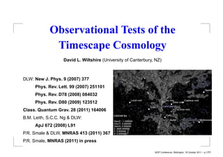
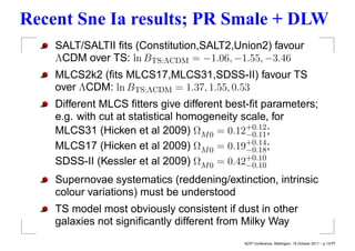
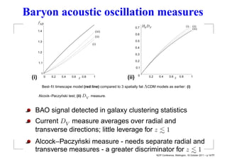
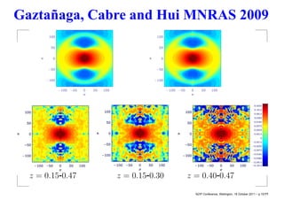
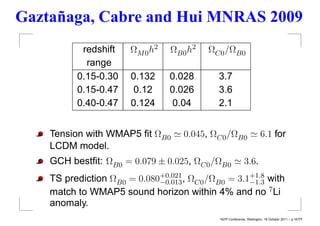
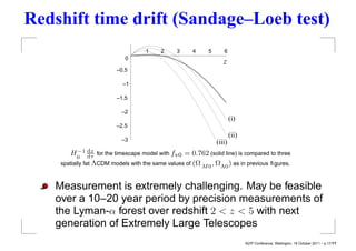
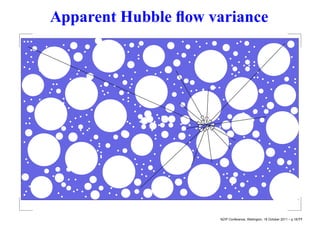
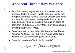
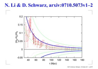
Observational Tests of the
             Timescape Cosmology
                   David L. Wiltshire (University of Canterbury, NZ)


DLW: New J. Phys. 9 (2007) 377
     Phys. Rev. Lett. 99 (2007) 251101
     Phys. Rev. D78 (2008) 084032
     Phys. Rev. D80 (2009) 123512
Class. Quantum Grav. 28 (2011) 164006
B.M. Leith, S.C.C. Ng & DLW:
     ApJ 672 (2008) L91
P.R. Smale & DLW, MNRAS 413 (2011) 367
P.R. Smale, MNRAS (2011) in press

                                                                NZIP Conference, Wellington, 18 October 2011 – p.1/??
Overview of timescape cosmology
Standard cosmology, with 22% non-baryonic dark
matter, 74% dark energy assumes universe expands as
smooth fluid, ignoring structures on scales
< 100h−1 Mpc
∼
Actual observed universe contains vast structures of
voids (most of volume), plus walls and filaments
containing galaxies
Timescape scenario - first principles model reanalysing
coarse-graining of “dust” in general relativity
Hypothesis: must understand nonlinear evolution with
backreaction, AND gravitational energy gradients within
the inhomogeneous geometry


                                       NZIP Conference, Wellington, 18 October 2011 – p.2/??
6df: voids & bubble walls (A. Fairall, UCT)


                              NZIP Conference, Wellington, 18 October 2011 – p.3/??
Within a statistically average cell


Need to consider relative position of observers over
scales of tens of Mpc over which δρ/ρ ∼ −1.
GR is a local theory: gradients in spatial curvature and
gravitational energy can lead to calibration differences
between our rulers and clocks and volume average
ones
                                         NZIP Conference, Wellington, 18 October 2011 – p.4/??
−10
                   Relative deceleration scale
      10 m/s 2
                                                                        0.12
       α
      1.2                                                               0.10
                                                                                   α /(Hc)
      1.0                                                               0.08


      0.8                                                               0.06

                                                                        0.04
      0.6

                                                                        0.02   α /(Hc)
      0.4

(i)         0     0.05     0.1   z 0.15    0.2    0.25
                                                                 (ii)          0      2        4    z      6           8         10
                Instantaneous relative volume deceleration of walls relative to volume average background
                                   q
                        ˙
            α = H0 c¯ w γ w /(
                    γ ¯              γ 2 − 1) computed for timescape model which best fits supernovae
                                      ¯w
            luminosity distances: (i) as absolute scale nearby; (ii) divided by Hubble parameter to large z .


        With α0 ∼ 7 × 10⁻¹¹ m s−2 and typically α ∼ 10−10 m s−2 for
        most of life of Universe, get 37% difference in
        calibration of volume average clocks relative to our own
                                                                                          NZIP Conference, Wellington, 18 October 2011 – p.5/??
Apparent cosmic acceleration
Volume average observer sees no apparent cosmic
acceleration
                      2 (1 − fv )2
                  q=
                  ¯              2
                                   .
                       (2 + fv )
As t → ∞, fv → 1 and q → 0+ .
                     ¯
A wall observer registers apparent cosmic acceleration

              − (1 − fv ) (8fv 3 + 39fv 2 − 12fv − 8)
         q=                                                     ,
                                        2 2
                         4 + fv + 4fv

Effective deceleration parameter starts at q ∼ 1 , for
                                               2
small fv ; changes sign when fv = 0.58670773 . . ., and
approaches q → 0− at late times.
                                              NZIP Conference, Wellington, 18 October 2011 – p.6/??
Cosmic coincidence problem solved
 Spatial curvature gradients largely responsible for
 gravitational energy gradient giving clock rate variance.
 Apparent acceleration starts when voids start to open.


                                          NZIP Conference, Wellington, 18 October 2011 – p.7/??
Best fit parameters
Hubble constant H0 + ∆H0 = 61.7+1.2 km/s/Mpc
                               −1.1
                                       +0.12
present void volume fraction fv0 = 0.76−0.09
                       ¯
bare density parameter ΩM 0 = 0.125+0.060
                                   −0.069

dressed density parameter ΩM 0 = 0.33+0.11
                                     −0.16
non–baryonic dark matter / baryonic matter mass ratio
 ¯      ¯     ¯
(ΩM 0 − ΩB0 )/ΩB0 = 3.1+2.5
                       −2.4
                     ¯
bare Hubble constant H 0 = 48.2+2.0 km/s/Mpc
                               −2.4

mean phenomenological lapse function γ 0 = 1.381+0.061
                                     ¯          −0.046
                                   +0.0120
deceleration parameter q0 = −0.0428−0.0002
wall age universe τ0 = 14.7+0.7 Gyr
                           −0.5
                                         NZIP Conference, Wellington, 18 October 2011 – p.8/??
Key observational tests


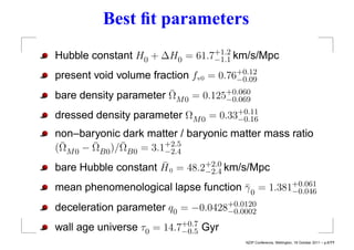
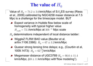
Best–fit parameters: H0 = 61.7+1.2 km/s/Mpc, Ωm = 0.33+0.11
                                −1.1                     −0.16
(1σ errors for SneIa only) [Leith, Ng & Wiltshire, ApJ 672
(2008) L91]
                                             NZIP Conference, Wellington, 18 October 2011 – p.9/??
Test 1: SneIa luminosity distances
        48
        46
        44
        42
        40
    µ

        38
        36
        34
        32
        30
          0      0.5      1        1.5                2
                          z
 Type Ia supernovae of Riess 2007 Gold data set fit with
 χ2 per degree of freedom = 0.9
 Type Ia supernovae of Hicken 2009 MLCS17 set fit with
 χ2 per degree of freedom = 1.08

                                         NZIP Conference, Wellington, 18 October 2011 – p.10/??
Dressed “comoving distance” D(z)
      H 0D                          (i)       3.5   H 0D                                                 (i)
 2                                   (ii)                                                                (ii)
                                   (iii)        3                                                        (iii)
1.5                                           2.5
                           1

                                                2
  1
                                              1.5

                                                1
0.5
                                              0.5
                          0             1
                                    z
 0       1       2   3    4    5   6            0      200   400      600          800       1000
                     z                                                z
               Best-fit timescape model (red line) compared to 3 spatially
             flat ΛCDM models: (i) best–fit to WMAP5 only (Ω = 0.75);
                                                              Λ
             (ii) joint WMAP5 + BAO + SneIa fit (Ω = 0.72);
                                                     Λ
             (iii) best flat fit to (Riess07) SneIa only (Ω = 0.66).
                                                         Λ

        Three different tests with hints of tension with ΛCDM
        agree well with TS model.
                                                             NZIP Conference, Wellington, 18 October 2011 – p.11/??
Supernovae systematics
                      Gold (167 SneIa)                             SDSS−II 1st year (272 SneIa)
      0.7                                               0.7

      0.6                                               0.6

      0.5                                               0.5

      0.4                                               0.4
Ωm0


                                                   m0
                                                   Ω
      0.3                                               0.3

      0.2                                               0.2

      0.1                                               0.1

       0                                                 0
            56   58     60    62    64   66   68              56    58     60    62        64       66       68
                             H0                                                 H0

                  MLCS17 (219 SneIa)                                   MLCS31 (219 SneIa)


      0.6                                               0.6

      0.5                                               0.5

      0.4                                               0.4
Ωm0


                                                   m0
                                                   Ω
      0.3                                               0.3

      0.2                                               0.2

      0.1                                               0.1

       0                                                 0
            56   58     60    62    64   66   68              56    58     60    62        64       66       68
                             H0                                                 H0
                                                                                NZIP Conference, Wellington, 18 October 2011 – p.12/??
Recent Sne Ia results; PR Smale + DLW
    SALT/SALTII fits (Constitution,SALT2,Union2) favour
    ΛCDM over TS: ln BTS:ΛCDM = −1.06, −1.55, −3.46
    MLCS2k2 (fits MLCS17,MLCS31,SDSS-II) favour TS
    over ΛCDM: ln BTS:ΛCDM = 1.37, 1.55, 0.53
    Different MLCS fitters give different best-fit parameters;
    e.g. with cut at statistical homogeneity scale, for
    MLCS31 (Hicken et al 2009) ΩM 0 = 0.12+0.12 ;
                                              −0.11
    MLCS17 (Hicken et al 2009) ΩM 0 = 0.19+0.14 ;
                                              −0.18
    SDSS-II (Kessler et al 2009) ΩM 0 = 0.42+0.10
                                              −0.10
    Supernovae systematics (reddening/extinction, intrinsic
    colour variations) must be understood
    TS model most obviously consistent if dust in other
    galaxies not significantly different from Milky Way
                                            NZIP Conference, Wellington, 18 October 2011 – p.13/??
Baryon acoustic oscillation measures
       f AP
                                                                   0.7   H0 D V                               (i)   (ii)
                                                                                                                    (iii)
       1.4                                      (iii)
                                                                   0.6
                                                (ii)
       1.3                                                         0.5
                                              (i)
                                                                   0.4
       1.2
                                                                   0.3

                                                                   0.2
       1.1
                                                                   0.1
         1
                                                                     0
 (i)          0   0.2   0.4   0.6   z   0.8    1            (ii)             0.2     0.4      0.6   z   0.8         1


         Best-fit timescape model (red line) compared to 3 spatially flat ΛCDM models as earlier: (i)

                   nski test; (ii) DV measure.
       Alcock–Paczy´


   BAO signal detected in galaxy clustering statistics
   Current DV measure averages over radial and
                                                <
   transverse directions; little leverage for z ∼ 1
   Alcock–Paczy´nski measure - needs separate radial and
                                                       <
   transverse measures - a greater discriminator for z ∼ 1
                                                                                   NZIP Conference, Wellington, 18 October 2011 – p.14/??
Gaztañaga, Cabre and Hui MNRAS 2009


  z = 0.15-0.47   z = 0.15-0.30   z = 0.40-0.47

                                    NZIP Conference, Wellington, 18 October 2011 – p.15/??
Gaztañaga, Cabre and Hui MNRAS 2009
           redshift    Ω M 0 h2   ΩB0 h2   ΩC0 /ΩB0
            range
          0.15-0.30    0.132      0.028      3.7
          0.15-0.47    0.12       0.026      3.6
          0.40-0.47    0.124       0.04      2.1


    Tension with WMAP5 fit ΩB0        0.045, ΩC0 /ΩB0                   6.1 for
    LCDM model.
    GCH bestfit: ΩB0 = 0.079 ± 0.025, ΩC0 /ΩB0               3.6.
    TS prediction ΩB0 = 0.080+0.021 , ΩC0 /ΩB0 = 3.1+1.8 with
                             −0.013                 −1.3
    match to WMAP5 sound horizon within 4% and no 7 Li
    anomaly.
                                             NZIP Conference, Wellington, 18 October 2011 – p.16/??
Redshift time drift (Sandage–Loeb test)
                                    1    2     3     4     5      6
                            0
                                                                  z
                         –0.5

                           –1

                         –1.5

                           –2
                                                                       (i)
                         –2.5
                                                                       (ii)
                           –3                                  (iii)
           −1 dz
       H0 dτ for the timescape model with fv0 = 0.762 (solid line) is compared to three
    spatially flat ΛCDM models with the same values of (Ω M 0 , ΩΛ0 ) as in previous figures.


   Measurement is extremely challenging. May be feasible
   over a 10–20 year period by precision measurements of
   the Lyman-α forest over redshift 2 < z < 5 with next
   generation of Extremely Large Telescopes
                                                                              NZIP Conference, Wellington, 18 October 2011 – p.17/??
Apparent Hubble flow variance


                     NZIP Conference, Wellington, 18 October 2011 – p.18/??
Apparent Hubble flow variance
As voids occupy largest volume of space expect to
measure higher average Hubble constant locally until
the global average relative volumes of walls and voids
are sampled at scale of homogeneity; thus expect
maximum H0 value for isotropic average on scale of
dominant void diameter, 30h−1 Mpc, then decreasing til
levelling out by 100h−1 Mpc.
Consistent with a Hubble bubble feature (Jha, Riess,
Kirshner ApJ 659, 122 (2007)); or “large scale flows”
with certain characteristics (cf Watkins et al).
Expected maximum “bulk dipole velocity”

                    ¯         30
       vpec =   ( 3H0
                  2     − H0 ) Mpc = 510+210 km/s
                              h         −260

                                         NZIP Conference, Wellington, 18 October 2011 – p.19/??
N. Li & D. Schwarz, arxiv:0710.5073v1–2

                 0.2


             0.15
    (HD-H0)/H0


                 0.1


             0.05


                  0


          -0.05
                       40   60   80   100       120   140         160              180
                                      r (Mpc)
                                                        NZIP Conference, Wellington, 18 October 2011 – p.20/??
PR Smale + DLW, in preparation


                      NZIP Conference, Wellington, 18 October 2011 – p.21/??
The value of H0
Value of H0 = 74.2 ± 3.6 km/s/Mpc of SH0 ES survey (Riess
et al., 2009) calibrated by NGC4258 maser distance at 7.5
Mpc is a challenge for the timescape model. BUT
   Expect variance in Hubble flow below scale of
   homogeneity with typical higher value
   Hvw0 = 72.3 km/s/Mpc at 30h−1 Mpc scale
H0 determinations independent of local distance ladder:
   WiggleZ FLRW BAO value (Beutler et al,
   arXiv:1106.3366): H0 = 67 ± 3.2 km/s/Mpc
   Quasar strong lensing time delays; e.g., (Courbin et al,
   1009.1473): H0 = 62+6 km/s/Mpc
                       −4
   Megamaser distance of UGC3789 H0 = 66.6 ± 11.4
   km/s/Mpc, (69 ± 11 km/s/Mpc with“flow modeling”).
                                           NZIP Conference, Wellington, 18 October 2011 – p.22/??
Summary
Apparent cosmic acceleration can be understood purely
within general relativity; by (i) treating geometry of
universe more realistically; (ii) understanding
fundamental aspects of general relativity of statistical
description of general relativity which have not been
fully explored – quasi–local gravitational energy,
of gradients in spatial curvature etc.
Extra ingredients – regional averages etc – go beyond
conventional applications of general relativity
Description of spacetime as a causal relational
structure – retains principles consistent with GR
Many details – averaging scheme etc – may change,
but fundamental questions remain in any approach


                                        NZIP Conference, Wellington, 18 October 2011 – p.23/??
Outlook
Other work
   Several observational tests (Alcock-Paczynski test,
   Clarkson, Bassett and Lu test, redshift time drift etc)
   discussed in PRD 80 (2009) 123512
Work in progress
                 ´
   Adapting Korzynski’s “covariant coarse-graining”
   approach to more rigorously define regional averages
   (with James Duley)
   Analysis of variance of Hubble flow in style of Li and
   Schwarz on large datasets (with Peter Smale)
   Full analysis of CMB anisotropy spectrum in timescape
   model (with Ahsan Nazer)


                                            NZIP Conference, Wellington, 18 October 2011 – p.24/??

16.40 o10 d wiltshire

  • 1.
    Observational Tests ofthe Timescape Cosmology David L. Wiltshire (University of Canterbury, NZ) DLW: New J. Phys. 9 (2007) 377 Phys. Rev. Lett. 99 (2007) 251101 Phys. Rev. D78 (2008) 084032 Phys. Rev. D80 (2009) 123512 Class. Quantum Grav. 28 (2011) 164006 B.M. Leith, S.C.C. Ng & DLW: ApJ 672 (2008) L91 P.R. Smale & DLW, MNRAS 413 (2011) 367 P.R. Smale, MNRAS (2011) in press NZIP Conference, Wellington, 18 October 2011 – p.1/??
  • 2.
    Overview of timescapecosmology Standard cosmology, with 22% non-baryonic dark matter, 74% dark energy assumes universe expands as smooth fluid, ignoring structures on scales < 100h−1 Mpc ∼ Actual observed universe contains vast structures of voids (most of volume), plus walls and filaments containing galaxies Timescape scenario - first principles model reanalysing coarse-graining of “dust” in general relativity Hypothesis: must understand nonlinear evolution with backreaction, AND gravitational energy gradients within the inhomogeneous geometry NZIP Conference, Wellington, 18 October 2011 – p.2/??
  • 3.
    6df: voids &bubble walls (A. Fairall, UCT) NZIP Conference, Wellington, 18 October 2011 – p.3/??
  • 4.
    Within a statisticallyaverage cell Need to consider relative position of observers over scales of tens of Mpc over which δρ/ρ ∼ −1. GR is a local theory: gradients in spatial curvature and gravitational energy can lead to calibration differences between our rulers and clocks and volume average ones NZIP Conference, Wellington, 18 October 2011 – p.4/??
  • 5.
    −10 Relative deceleration scale 10 m/s 2 0.12 α 1.2 0.10 α /(Hc) 1.0 0.08 0.8 0.06 0.04 0.6 0.02 α /(Hc) 0.4 (i) 0 0.05 0.1 z 0.15 0.2 0.25 (ii) 0 2 4 z 6 8 10 Instantaneous relative volume deceleration of walls relative to volume average background q ˙ α = H0 c¯ w γ w /( γ ¯ γ 2 − 1) computed for timescape model which best fits supernovae ¯w luminosity distances: (i) as absolute scale nearby; (ii) divided by Hubble parameter to large z . With α0 ∼ 7 × 10⁻¹¹ m s−2 and typically α ∼ 10−10 m s−2 for most of life of Universe, get 37% difference in calibration of volume average clocks relative to our own NZIP Conference, Wellington, 18 October 2011 – p.5/??
  • 6.
    Apparent cosmic acceleration Volumeaverage observer sees no apparent cosmic acceleration 2 (1 − fv )2 q= ¯ 2 . (2 + fv ) As t → ∞, fv → 1 and q → 0+ . ¯ A wall observer registers apparent cosmic acceleration − (1 − fv ) (8fv 3 + 39fv 2 − 12fv − 8) q= , 2 2 4 + fv + 4fv Effective deceleration parameter starts at q ∼ 1 , for 2 small fv ; changes sign when fv = 0.58670773 . . ., and approaches q → 0− at late times. NZIP Conference, Wellington, 18 October 2011 – p.6/??
  • 7.
    Cosmic coincidence problemsolved Spatial curvature gradients largely responsible for gravitational energy gradient giving clock rate variance. Apparent acceleration starts when voids start to open. NZIP Conference, Wellington, 18 October 2011 – p.7/??
  • 8.
    Best fit parameters Hubbleconstant H0 + ∆H0 = 61.7+1.2 km/s/Mpc −1.1 +0.12 present void volume fraction fv0 = 0.76−0.09 ¯ bare density parameter ΩM 0 = 0.125+0.060 −0.069 dressed density parameter ΩM 0 = 0.33+0.11 −0.16 non–baryonic dark matter / baryonic matter mass ratio ¯ ¯ ¯ (ΩM 0 − ΩB0 )/ΩB0 = 3.1+2.5 −2.4 ¯ bare Hubble constant H 0 = 48.2+2.0 km/s/Mpc −2.4 mean phenomenological lapse function γ 0 = 1.381+0.061 ¯ −0.046 +0.0120 deceleration parameter q0 = −0.0428−0.0002 wall age universe τ0 = 14.7+0.7 Gyr −0.5 NZIP Conference, Wellington, 18 October 2011 – p.8/??
  • 9.
    Key observational tests Best–fitparameters: H0 = 61.7+1.2 km/s/Mpc, Ωm = 0.33+0.11 −1.1 −0.16 (1σ errors for SneIa only) [Leith, Ng & Wiltshire, ApJ 672 (2008) L91] NZIP Conference, Wellington, 18 October 2011 – p.9/??
  • 10.
    Test 1: SneIaluminosity distances 48 46 44 42 40 µ 38 36 34 32 30 0 0.5 1 1.5 2 z Type Ia supernovae of Riess 2007 Gold data set fit with χ2 per degree of freedom = 0.9 Type Ia supernovae of Hicken 2009 MLCS17 set fit with χ2 per degree of freedom = 1.08 NZIP Conference, Wellington, 18 October 2011 – p.10/??
  • 11.
    Dressed “comoving distance”D(z) H 0D (i) 3.5 H 0D (i) 2 (ii) (ii) (iii) 3 (iii) 1.5 2.5 1 2 1 1.5 1 0.5 0.5 0 1 z 0 1 2 3 4 5 6 0 200 400 600 800 1000 z z Best-fit timescape model (red line) compared to 3 spatially flat ΛCDM models: (i) best–fit to WMAP5 only (Ω = 0.75); Λ (ii) joint WMAP5 + BAO + SneIa fit (Ω = 0.72); Λ (iii) best flat fit to (Riess07) SneIa only (Ω = 0.66). Λ Three different tests with hints of tension with ΛCDM agree well with TS model. NZIP Conference, Wellington, 18 October 2011 – p.11/??
  • 12.
    Supernovae systematics Gold (167 SneIa) SDSS−II 1st year (272 SneIa) 0.7 0.7 0.6 0.6 0.5 0.5 0.4 0.4 Ωm0 m0 Ω 0.3 0.3 0.2 0.2 0.1 0.1 0 0 56 58 60 62 64 66 68 56 58 60 62 64 66 68 H0 H0 MLCS17 (219 SneIa) MLCS31 (219 SneIa) 0.6 0.6 0.5 0.5 0.4 0.4 Ωm0 m0 Ω 0.3 0.3 0.2 0.2 0.1 0.1 0 0 56 58 60 62 64 66 68 56 58 60 62 64 66 68 H0 H0 NZIP Conference, Wellington, 18 October 2011 – p.12/??
  • 13.
    Recent Sne Iaresults; PR Smale + DLW SALT/SALTII fits (Constitution,SALT2,Union2) favour ΛCDM over TS: ln BTS:ΛCDM = −1.06, −1.55, −3.46 MLCS2k2 (fits MLCS17,MLCS31,SDSS-II) favour TS over ΛCDM: ln BTS:ΛCDM = 1.37, 1.55, 0.53 Different MLCS fitters give different best-fit parameters; e.g. with cut at statistical homogeneity scale, for MLCS31 (Hicken et al 2009) ΩM 0 = 0.12+0.12 ; −0.11 MLCS17 (Hicken et al 2009) ΩM 0 = 0.19+0.14 ; −0.18 SDSS-II (Kessler et al 2009) ΩM 0 = 0.42+0.10 −0.10 Supernovae systematics (reddening/extinction, intrinsic colour variations) must be understood TS model most obviously consistent if dust in other galaxies not significantly different from Milky Way NZIP Conference, Wellington, 18 October 2011 – p.13/??
  • 14.
    Baryon acoustic oscillationmeasures f AP 0.7 H0 D V (i) (ii) (iii) 1.4 (iii) 0.6 (ii) 1.3 0.5 (i) 0.4 1.2 0.3 0.2 1.1 0.1 1 0 (i) 0 0.2 0.4 0.6 z 0.8 1 (ii) 0.2 0.4 0.6 z 0.8 1 Best-fit timescape model (red line) compared to 3 spatially flat ΛCDM models as earlier: (i) nski test; (ii) DV measure. Alcock–Paczy´ BAO signal detected in galaxy clustering statistics Current DV measure averages over radial and < transverse directions; little leverage for z ∼ 1 Alcock–Paczy´nski measure - needs separate radial and < transverse measures - a greater discriminator for z ∼ 1 NZIP Conference, Wellington, 18 October 2011 – p.14/??
  • 15.
    Gaztañaga, Cabre andHui MNRAS 2009 z = 0.15-0.47 z = 0.15-0.30 z = 0.40-0.47 NZIP Conference, Wellington, 18 October 2011 – p.15/??
  • 16.
    Gaztañaga, Cabre andHui MNRAS 2009 redshift Ω M 0 h2 ΩB0 h2 ΩC0 /ΩB0 range 0.15-0.30 0.132 0.028 3.7 0.15-0.47 0.12 0.026 3.6 0.40-0.47 0.124 0.04 2.1 Tension with WMAP5 fit ΩB0 0.045, ΩC0 /ΩB0 6.1 for LCDM model. GCH bestfit: ΩB0 = 0.079 ± 0.025, ΩC0 /ΩB0 3.6. TS prediction ΩB0 = 0.080+0.021 , ΩC0 /ΩB0 = 3.1+1.8 with −0.013 −1.3 match to WMAP5 sound horizon within 4% and no 7 Li anomaly. NZIP Conference, Wellington, 18 October 2011 – p.16/??
  • 17.
    Redshift time drift(Sandage–Loeb test) 1 2 3 4 5 6 0 z –0.5 –1 –1.5 –2 (i) –2.5 (ii) –3 (iii) −1 dz H0 dτ for the timescape model with fv0 = 0.762 (solid line) is compared to three spatially flat ΛCDM models with the same values of (Ω M 0 , ΩΛ0 ) as in previous figures. Measurement is extremely challenging. May be feasible over a 10–20 year period by precision measurements of the Lyman-α forest over redshift 2 < z < 5 with next generation of Extremely Large Telescopes NZIP Conference, Wellington, 18 October 2011 – p.17/??
  • 18.
    Apparent Hubble flowvariance NZIP Conference, Wellington, 18 October 2011 – p.18/??
  • 19.
    Apparent Hubble flowvariance As voids occupy largest volume of space expect to measure higher average Hubble constant locally until the global average relative volumes of walls and voids are sampled at scale of homogeneity; thus expect maximum H0 value for isotropic average on scale of dominant void diameter, 30h−1 Mpc, then decreasing til levelling out by 100h−1 Mpc. Consistent with a Hubble bubble feature (Jha, Riess, Kirshner ApJ 659, 122 (2007)); or “large scale flows” with certain characteristics (cf Watkins et al). Expected maximum “bulk dipole velocity” ¯ 30 vpec = ( 3H0 2 − H0 ) Mpc = 510+210 km/s h −260 NZIP Conference, Wellington, 18 October 2011 – p.19/??
  • 20.
    N. Li &D. Schwarz, arxiv:0710.5073v1–2 0.2 0.15 (HD-H0)/H0 0.1 0.05 0 -0.05 40 60 80 100 120 140 160 180 r (Mpc) NZIP Conference, Wellington, 18 October 2011 – p.20/??
  • 21.
    PR Smale +DLW, in preparation NZIP Conference, Wellington, 18 October 2011 – p.21/??
  • 22.
    The value ofH0 Value of H0 = 74.2 ± 3.6 km/s/Mpc of SH0 ES survey (Riess et al., 2009) calibrated by NGC4258 maser distance at 7.5 Mpc is a challenge for the timescape model. BUT Expect variance in Hubble flow below scale of homogeneity with typical higher value Hvw0 = 72.3 km/s/Mpc at 30h−1 Mpc scale H0 determinations independent of local distance ladder: WiggleZ FLRW BAO value (Beutler et al, arXiv:1106.3366): H0 = 67 ± 3.2 km/s/Mpc Quasar strong lensing time delays; e.g., (Courbin et al, 1009.1473): H0 = 62+6 km/s/Mpc −4 Megamaser distance of UGC3789 H0 = 66.6 ± 11.4 km/s/Mpc, (69 ± 11 km/s/Mpc with“flow modeling”). NZIP Conference, Wellington, 18 October 2011 – p.22/??
  • 23.
    Summary Apparent cosmic accelerationcan be understood purely within general relativity; by (i) treating geometry of universe more realistically; (ii) understanding fundamental aspects of general relativity of statistical description of general relativity which have not been fully explored – quasi–local gravitational energy, of gradients in spatial curvature etc. Extra ingredients – regional averages etc – go beyond conventional applications of general relativity Description of spacetime as a causal relational structure – retains principles consistent with GR Many details – averaging scheme etc – may change, but fundamental questions remain in any approach NZIP Conference, Wellington, 18 October 2011 – p.23/??
  • 24.
    Outlook Other work Several observational tests (Alcock-Paczynski test, Clarkson, Bassett and Lu test, redshift time drift etc) discussed in PRD 80 (2009) 123512 Work in progress ´ Adapting Korzynski’s “covariant coarse-graining” approach to more rigorously define regional averages (with James Duley) Analysis of variance of Hubble flow in style of Li and Schwarz on large datasets (with Peter Smale) Full analysis of CMB anisotropy spectrum in timescape model (with Ahsan Nazer) NZIP Conference, Wellington, 18 October 2011 – p.24/??