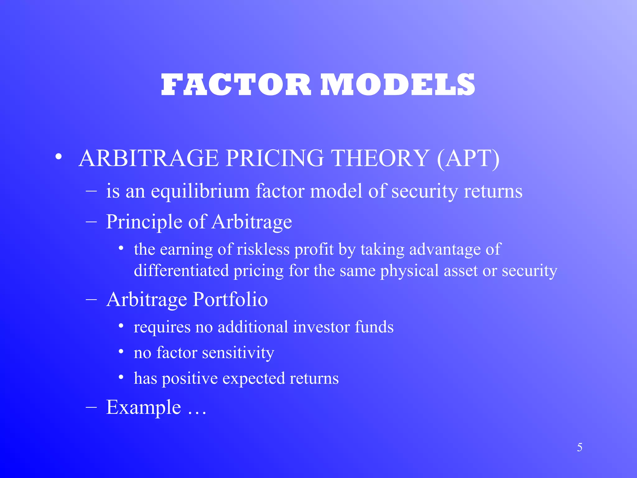
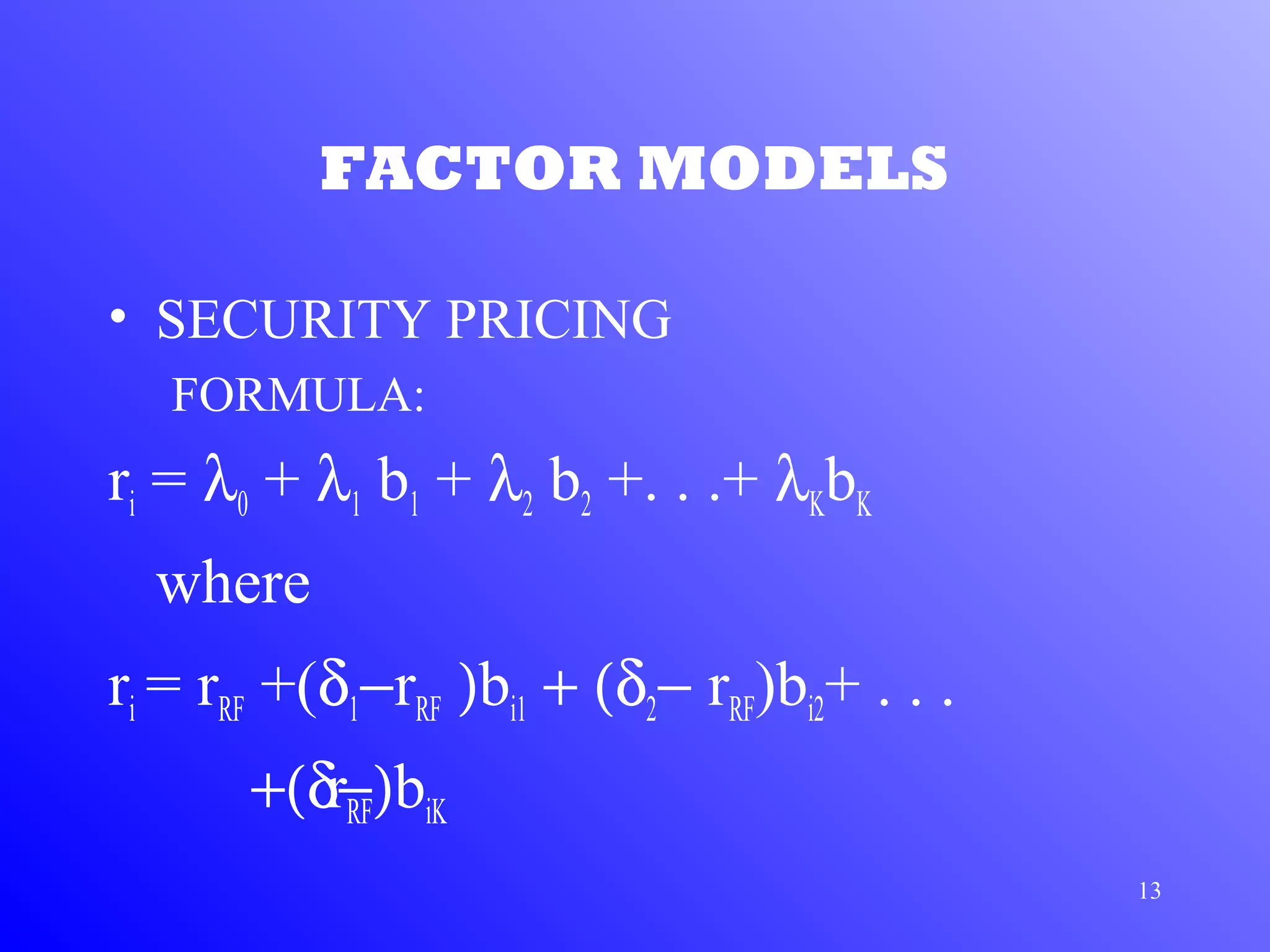
1) Arbitrage Pricing Theory (APT) is an equilibrium factor model that states a security's expected return is determined by its sensitivity to various macroeconomic factors.
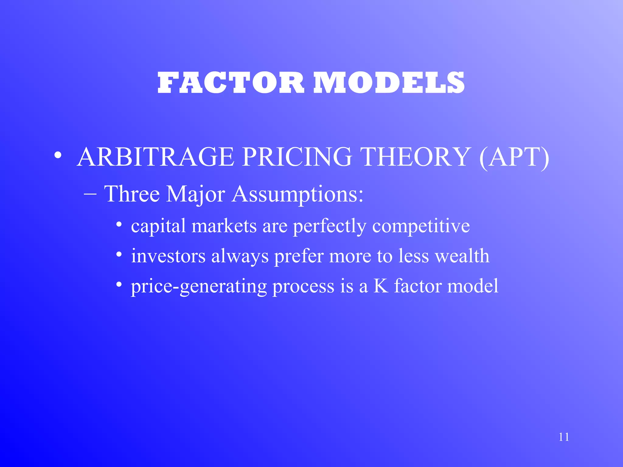
2) APT assumes capital markets are perfectly competitive and investors prefer more wealth to less. The price-generating process can be modeled as a multi-factor model.
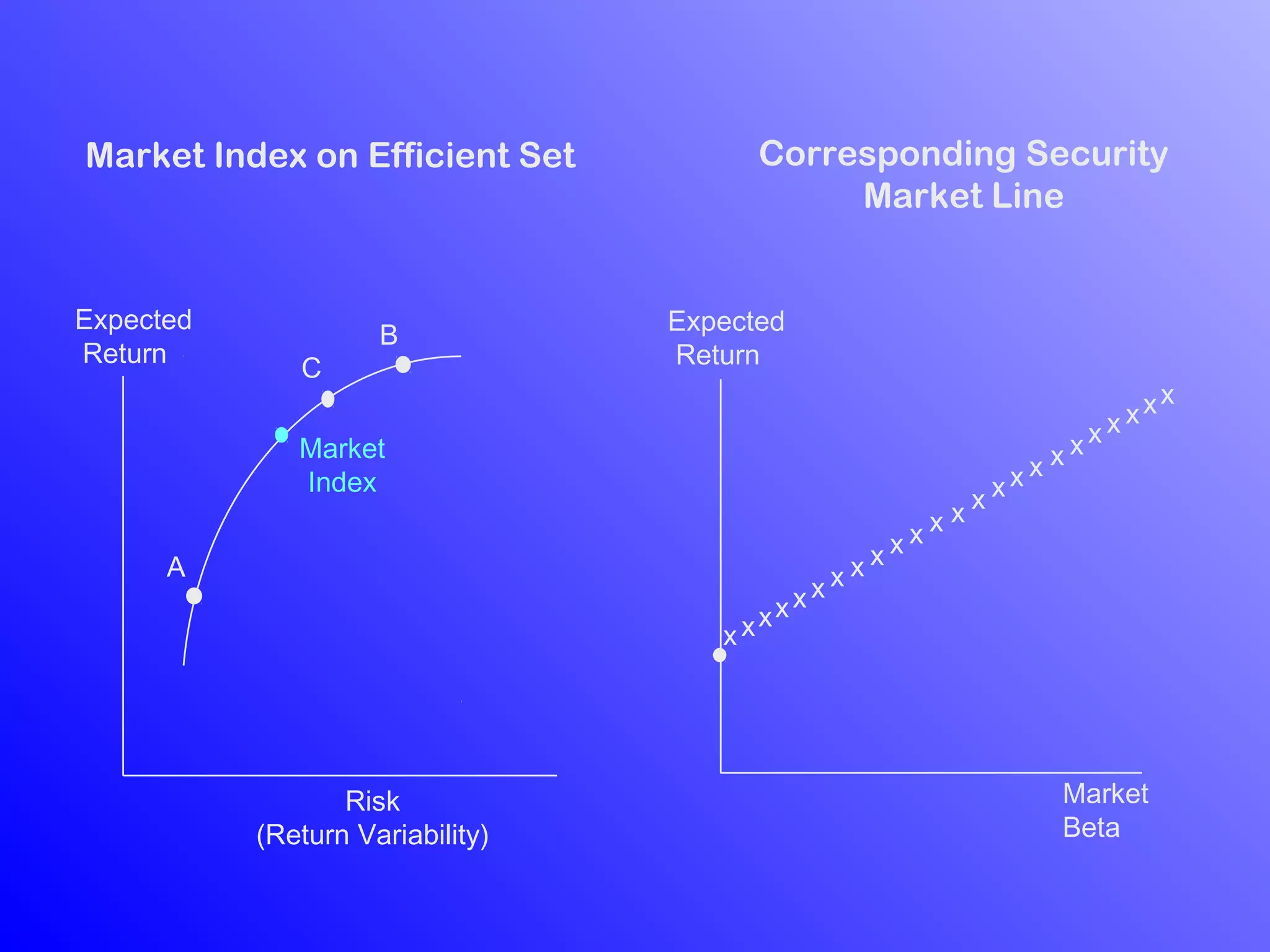
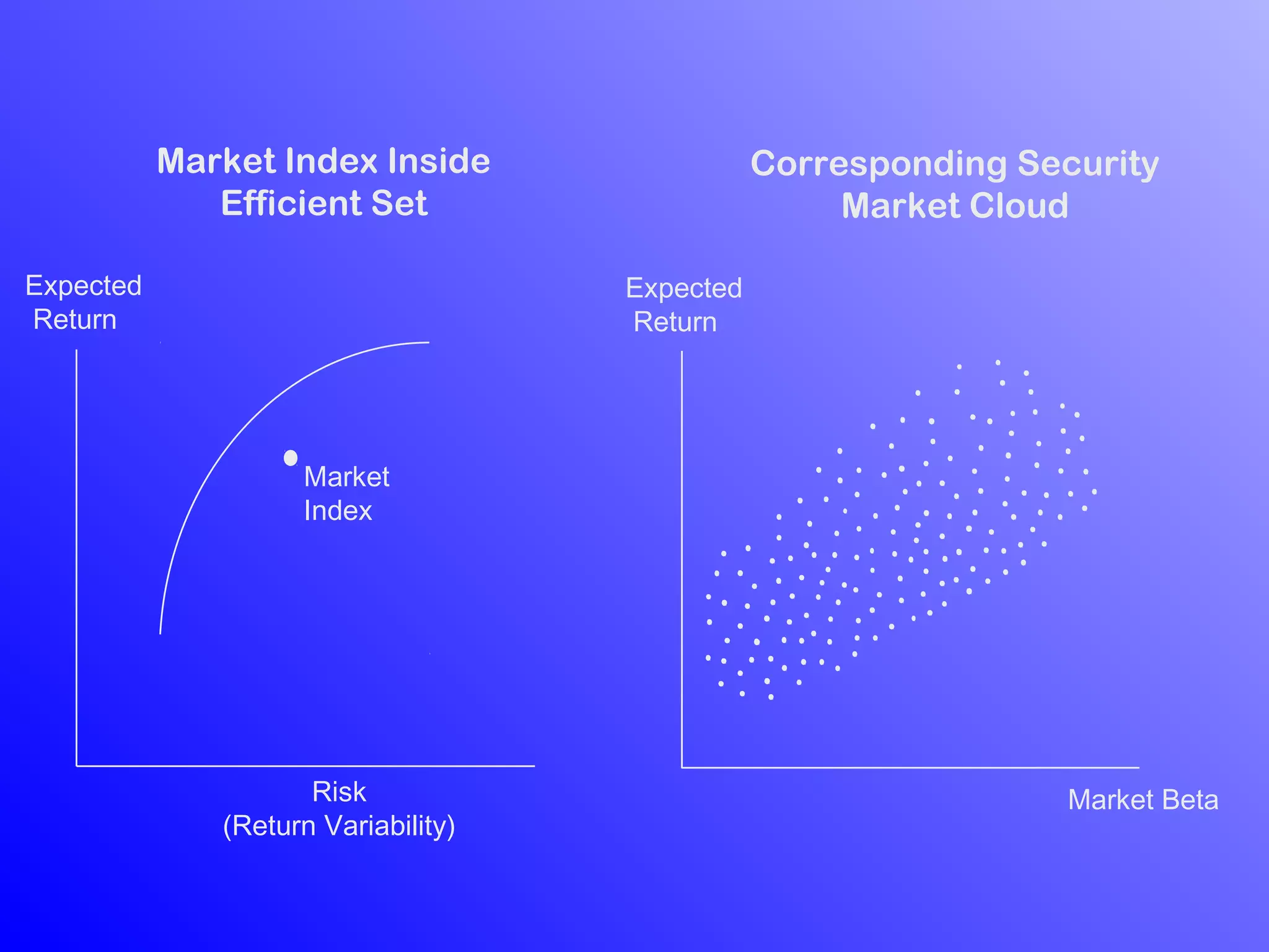
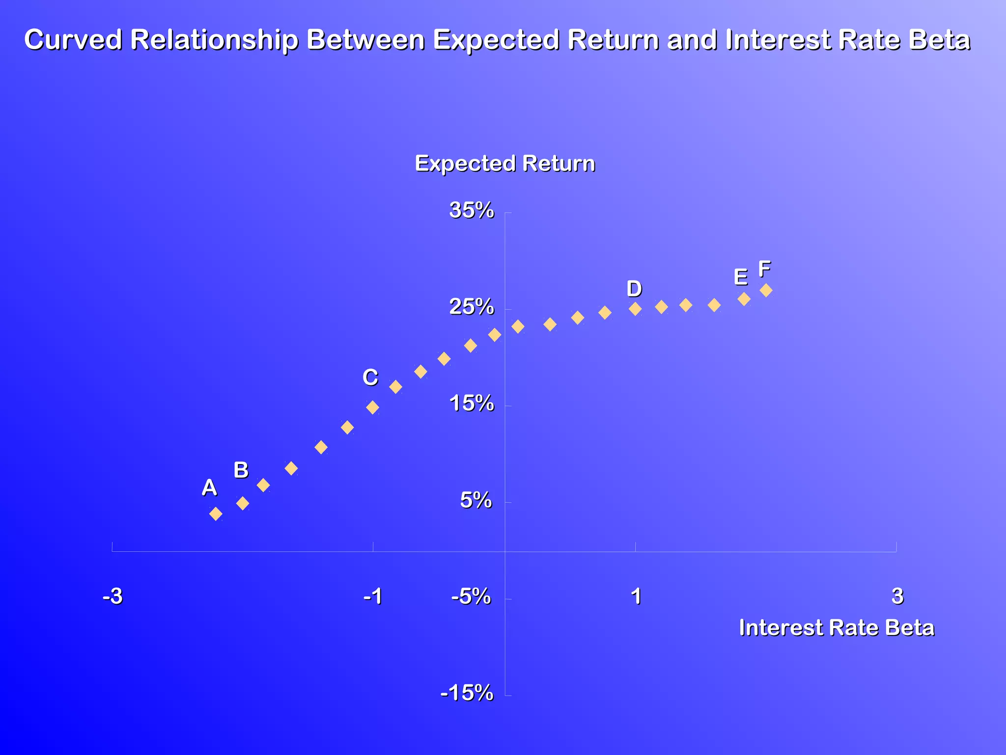
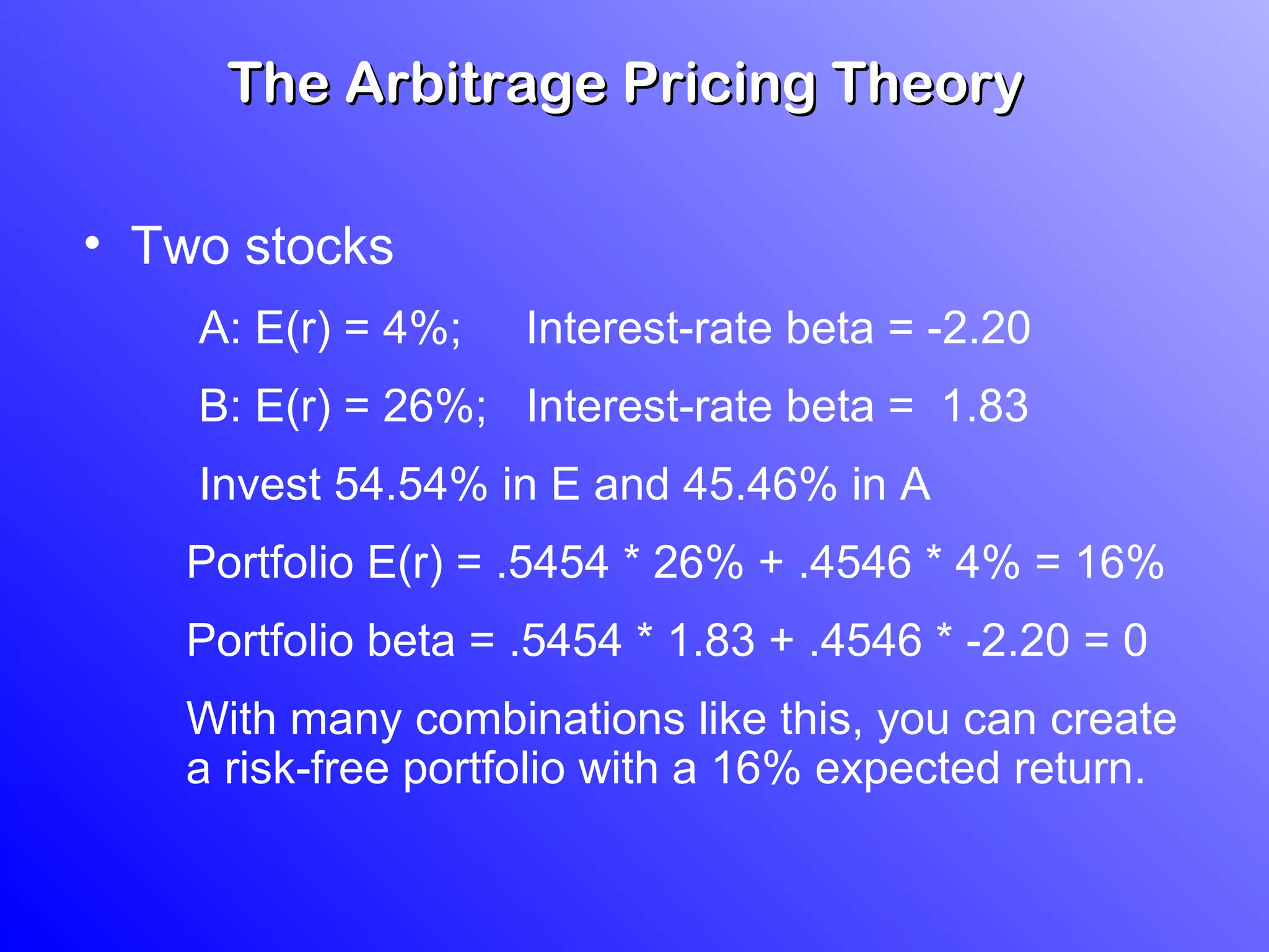
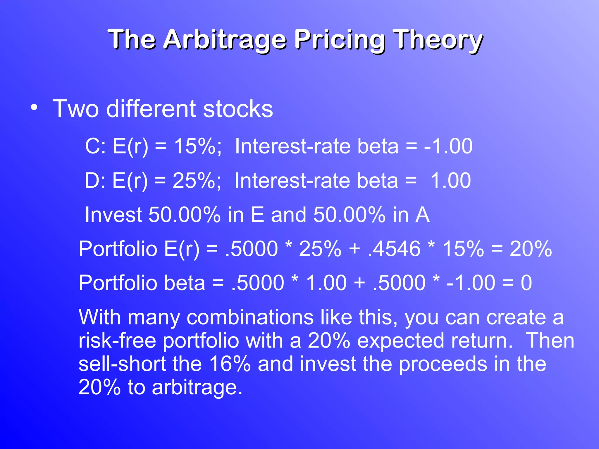
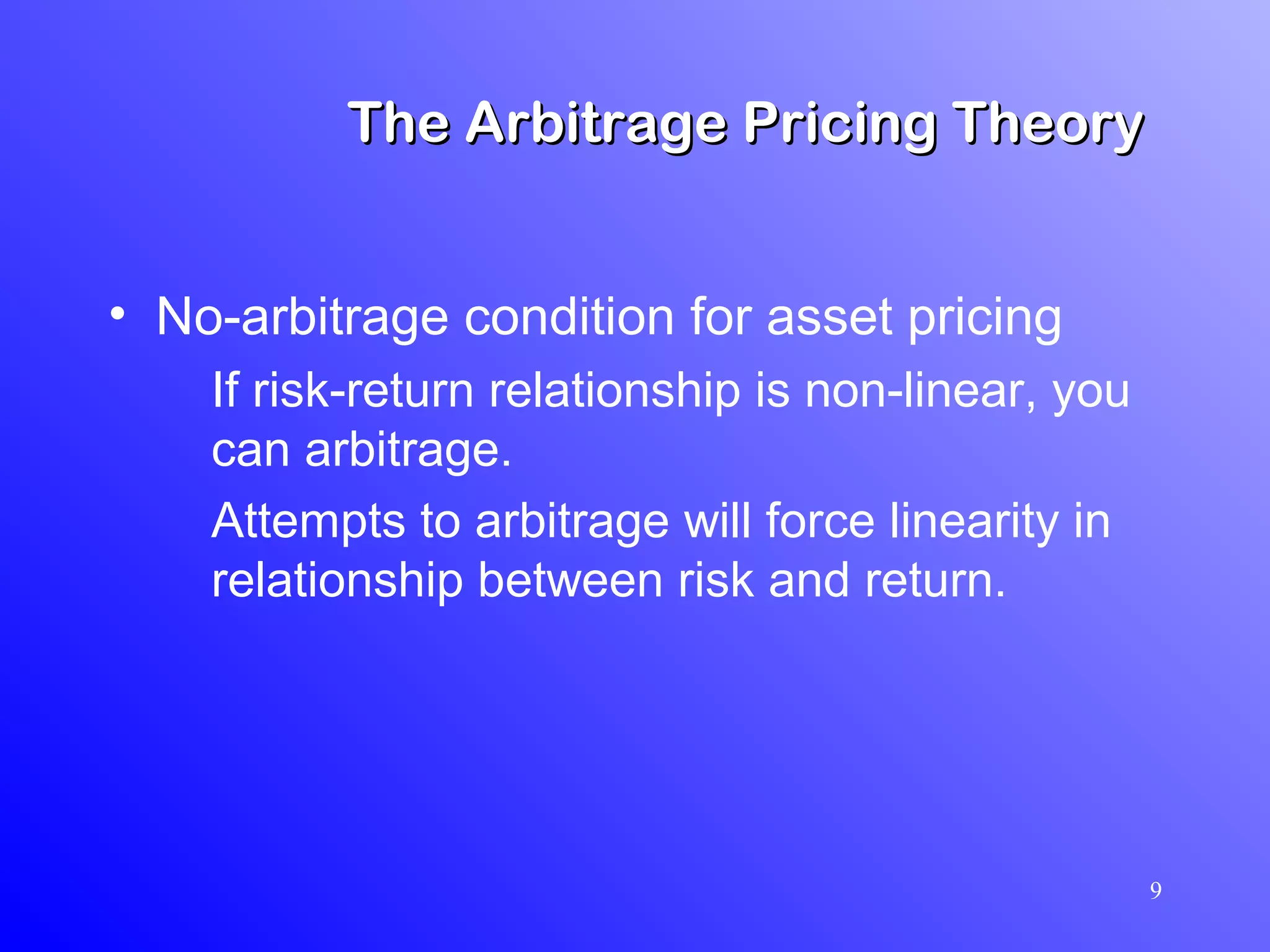
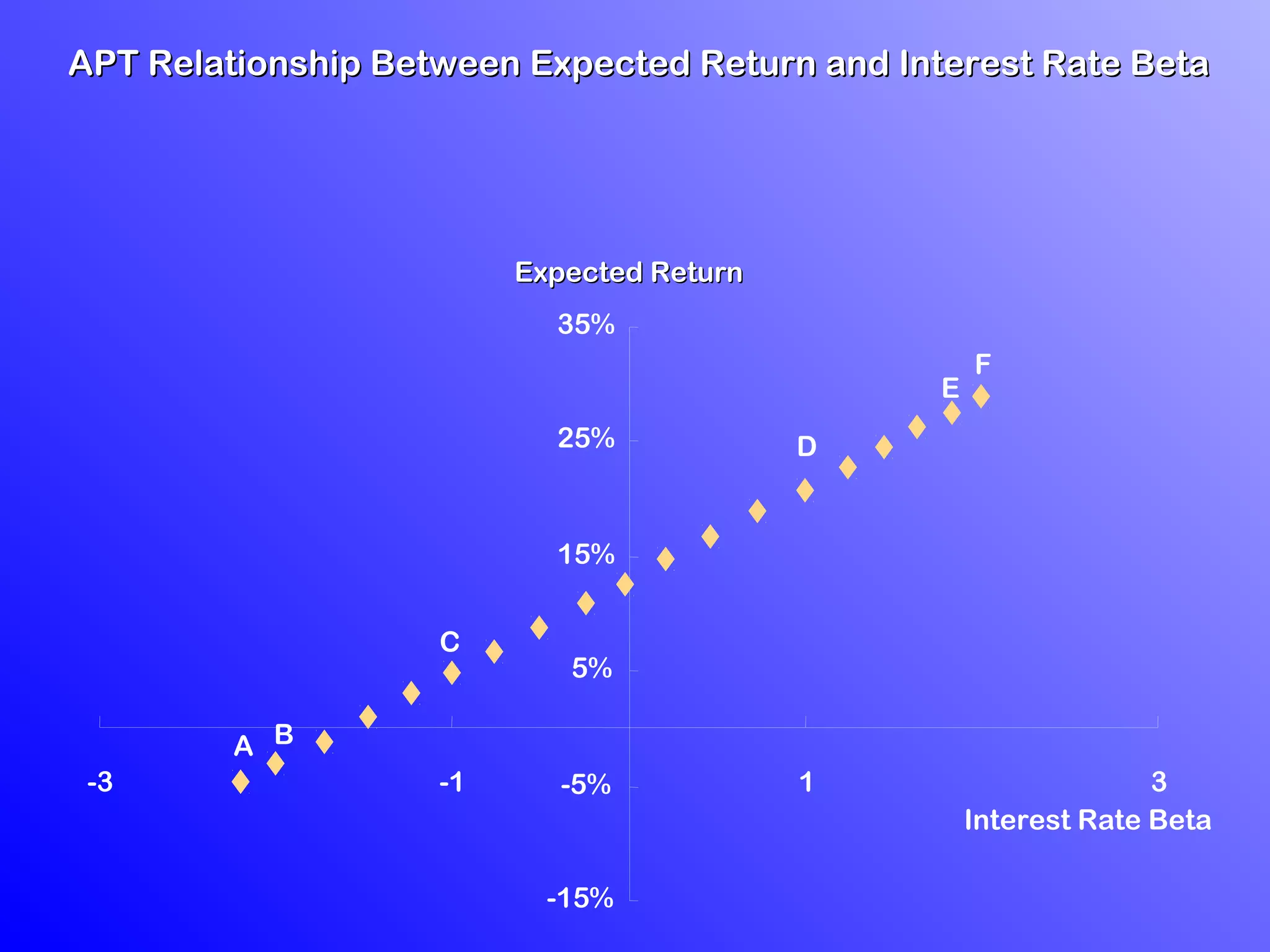
3) According to APT, if the risk-return relationship is non-linear, arbitrage opportunities exist as risk-free portfolios can be constructed with positive expected returns. Attempts to arbitrage will force the relationship between risk and return to become linear.