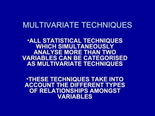
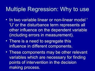
This document discusses multivariate techniques, specifically multiple regression. It defines multivariate techniques as those that analyze more than two variables simultaneously, accounting for relationships among variables. Multiple regression is described as a dependence method that uses one dependent variable and multiple independent variables. The document provides details on additive and multiplicative regression models, the matrix form of multiple regression equations, and assumptions of the technique. It also outlines how to interpret multiple regression output, including significance of slope coefficients and the adjusted R-squared statistic.

1. MULTIVARIATE TECHNIQUES
•ALL STATISTICAL TECHNIQUES
WHICH SIMULTANEOUSLY
ANALYSE MORE THAN TWO
VARIABLES CAN BE CATEGORISED
AS MULTIVARIATE TECHNIQUES
•THESE TECHNIQUES TAKE INTO
ACCOUNT THE DIFFERENT TYPES
OF RELATIONSHIPS AMONGST
VARIABLES

2. TYPES OF MUTIVARIATE TECHNIQUES
• ALL MULTIVARIATE TECHNIQUES ARE
BROADLY CLASSIFIED INTO TWO
CATEGORIES:
(I) DEPENDENCE METHODS
(II) INTEDEPENDENCE METHODS
• Several Variants of these methods are there
on the basis of the following
• (a) Number of dependent variables
• (b) The nature of data used in a model( with
reference to the scale of measurement)

3. Multivariate Techniques to be
discussed/used in this course
• Multiple Regression
(Both Additive and Multiplicative Models)
• Exploratory Factor Analysis
• Cluster Analysis

4. Multiple Regression
(Dependence methods)
• Multiple Regression is one of the important
Multivariate Techniques under the dependence
methods.
• In MR we have one dependent and more than
one independent variables.
• The dependent variables is in metric
measurement scale and the independent
variables are normally in metric scale but in
cases qualitative variables measured in nominal
scale could also be used with a specific
purpose.

5. Multiple Regression: Why to use
• In two variable linear or non-linear model '
'U' or the disturbance term represents all
other influence on the dependent variable
(including errors in measurement).
• There is a need to segregate this
influence in different components.
• These components may be other relevant
variables which are necessary for finding
points of intervention in the decision
making process.

6. Multiple Regression
The general form
• If we have specified a functional
relationship between 'Y' and several 'Xs'
Such as Y = ( X1,X2,X3,…..Xk) and have 'n'
observations, we may write the general form
of the Multiple Regression in different
ways such as linear or loglinear.
(Additive and Multiplicative regression
models have wide application in empirical
Research.)

7. Additive and Multiplicative
Regression Models
• Additive Regression Model
Y= b1 + b2 X2i+ b3X3i +….+ bkXki + Ui
This is used in estimation and forecasting.
Multiplicative Regression Model
Y = b1X2
b2
X3
b3 …
Xk
bk
Ui i= 1…n
Taking log of both sides we get a log linear regression
model.
Log Y = Log b1 + b2 LogX2i+…+ bk Log Xki + Ui
In this model, slopes are the respective elasticities
associated with a variable. This can be used to
estimate production functions where the slopes are
the input elasticities.

8. The matrix form of the Multiple Regression
• Since we have 'n' observations we can rewrite
the regression equation in matrix notation such
as the following
Y = X β + U
Where Y , B and U are a column vectors and X is a
matrix of order n x k.
If ei is the estimated ui , the equation can be
written as Y = X β + e and
∑ei
2
= e é (Is a function of β )
Minimizing this with respect to β would give
β^
= (X1
X)-1
X1
Y

9. Slope coefficients will be the Best Linear
Unbiased Estimates with respect to a set of
assumptions.
• Assumptions mostly relate to the variance
covariance matrix and the behavior of the
error term (u).
• One of the important assumptions relate to
the formula for calculating the slope
coefficients which suggests that (X1
X)-1
should exist.
• Therefore, one has to see that there is no
perfect collinearity between any pair of
variables.

10. The Correlation Table
• To examine the pair wise correlation between
variables one may examine the correlation
matrix.
• Trial and error methods is applied to arrive at
a set of independent variables that best
explain the dependent variables by the use
of several combinations of explanatory
variables and comparing the explanatory
power and the significance levels of the βi
s .Adjusted R2
may be considered in MR.

11. Interpretation of the Output
• DECISION POINTS AND INTERPRETATION:
1. 't' Values of β^¡ = β^¡ / SE of β¡
With the help of the sign and
significance levels conclusions on
relationship is arrived at.
2. R2
& Adjusted R2
(R bar Square).
R2
is a non-decreasing function of the
number of explanatory variable or
regressors present in the model.

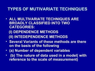
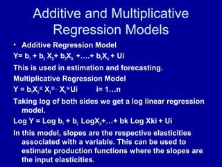
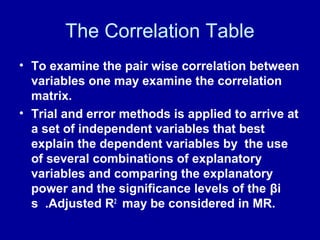
12. • Consider the Venn Diagram discussed earlier.
• If one increases the number of explanatory
variables one after the other R2
is expected to
increase (Not decrease)
• R2
is adjusted to the number of parameters in
the model. Hence, it is a better estimate of the
co-efficient of determination (Adjusted)
•The following formula is used to calculate the
Adjusted R2
•R2
= 1 – RSS/TSS or 1 - ∑ ui
2
/ ∑ yi
2
• Adjusted R2
= 1 – [∑ ui
2
/ (n-k)]/ ∑ yi
2
/ (n-1)
• Where k is the number of parameter including
the intercept term. ( See Page 217: 4th
Ed DNG)

13. Interpretation of the Output
• Comparing two R2
• The dependent variable and number of
• observation have to be the same.
• 3. Standardized Coefficients: They
indicate the relative importance of the
independent variables in explaining the
dependent variable.

14. Summary of Multiple Regression- An Example
(A Table can be computed as follows for comparison with
different combinations of independent variables)
Note: The figures in the parentheses are the significance
levels of the coefficients and the standardized coefficients
Dependen
t variable
Constant slope X1 SlopeX2 SlopeX3 SlopeX4 Adj R2
1 . Y 112.035
Std Coef
1.05
(0.01)
( 0.78)
0.087
(0.002)
(0.28)
1.009
(0.34)
(0.08)
0.009
(0.12)
(0.21)
0.82
2. Y …… …… …… x …….. …..
3. Y ……. …… ………. …….. x …

15. Assignment 3
• Groups will use time series and cross
section data in estimating the Multiple
Regression.
• Both additive and Multiplicative Models will
be estimated.
• Two /three combinations could be used after
examining the correlation table.
• The output may be summarized in a table.
• Ref: Basic Econometrics by DN Gujarati
• & Business Research Methods by P.Mishra