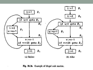
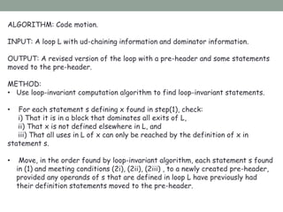
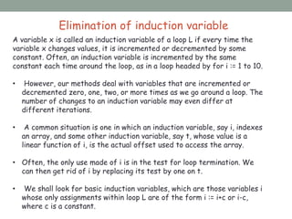
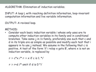
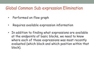
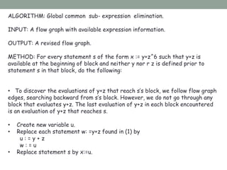
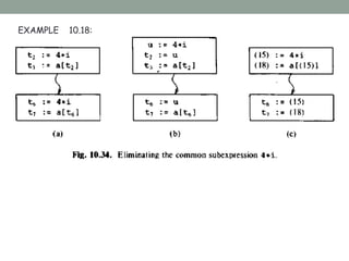
The document discusses techniques for improving code through transformations, including eliminating common subexpressions, copy propagation, detecting loop-invariant computations, performing code motion, and eliminating induction variables. Code transformations aim to reduce code size and running time by taking advantage of properties like invariant values to optimize programs without changing their meaning or output. Algorithms described include analyzing flow graphs, data flow, and control flow to identify optimization opportunities and apply transformations correctly and safely.

1. CODE – IMPROVING
TRANFORMATIONS
BY:
P.Vichitra
BP150513
IInd Msc[C.S]

2. Contents
Introduction
Elimination of Global Common Sub-expressions
Copy Propagation
Detection of Loop-Invariant Computations
Performing Code Motion
Alternative Code Motion Strategies
Maintaining Data-Flow Information After Code
Motion
Elimination of Induction Variables

3. What is code optimization?
• The code produced by the straight forward compiling
algorithms can often be made to run faster or take less
space or both.
• This improvement is achieved by program transformations
that are traditionally called optimizations.
• Machine independent optimizations are program
transformations that improve the target code without
taking into consideration any properties of the target
machine.
• Machine dependent optimizations are based on register
allocation and utilization of special machine-instruction
sequences.

4. Why Code-improving Transformation?
Code transformations are performed for a
variety of reasons among which are:
• To reduce the size of the code
• To reduce the running time of the
program
• To take advantage of machine idioms

5. Criteria for code improvement
transformations:
Simply stated , the best program transformations are
those that yield the most benefit for the least effort.
• The transformation must preserve the meaning of
programs. That is, the optimization must not change
the output produced by a program for a given input, or
cause an error.
• A transformation must, on the average, speed up
programs by a measurable amount.
• The transformation must be worth the effort.

6. Global Common Sub expression Elimination
• Performed on flow graph
• Requires available expression information
• In addition to finding what expressions are available
at the endpoints of basic blocks, we need to know
where each of those expressions was most recently
evaluated (which block and which position within that
block).

7. ALGORITHM: Global common sub- expression elimination.
INPUT: A flow graph with available expression information.
OUTPUT: A revised flow graph.
METHOD: For every statement s of the form x := y+z^6 such that y+z is
available at the beginning of block and neither y nor r z is defined prior to
statement s in that block, do the following:
• To discover the evaluations of y+z that reach s’s block, we follow flow graph
edges, searching backward from s’s block. However, we do not go through any
block that evaluates y+z. The last evaluation of y+z in each block encountered
is an evaluation of y+z that reaches s.
• Create new variable u.
• Replace each statement w: =y+z found in (1) by
u : = y + z
w : = u
• Replace statement s by x:=u.

8. EXAMPLE 10.18:

9. Copy Propagation
• Performed on flow graph.
• Given copy statement x=y and use w=x, we can replace w=x
with w=y only if the following conditions are met:
1. x=y must be the only definition of x reaching w=x
-This can be determined through ud-chains
2. There may be no definitions of y on any path from
x=y to w=x.
-Use iterative data flow analysis to solve this.
-Even, better, use iterative data flow analysis to solve both
problems at the same time.

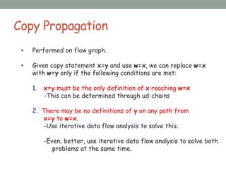
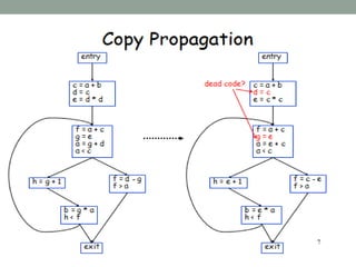
10. ALGORITHM: Copy propagation.
INPUT: a flow graph G, with ud-chains giving the definitions reaching
block B, and with c in[B] representing the solution to equations that is the
set of copies x:=y that reach block B along every path, with no assignment
to x or y following the last occurrence of x:=y on the path. We also need
ud-chains giving the uses of each definition.
OUTPUT: A revised flow graph.
METHOD: For each copy s : x:=y do the following:
• Determine those uses of x that are reached by this definition of
namely, s: x: =y.
• Determine whether for every use of x found in (1) , s is in c in[B],
where B is the block of this particular use, and moreover, no
definitions of x or y occur prior to this use of x within B. Recall that if
s is in c in[B]then s is the only definition of x that reaches B.
• If s meets the conditions of (2), then remove s and replace all uses of
x found in (1) by y.

12. Detection of loop-invariant computations
• Ud-chains can be used to detect those computations in a loop that are
loop-invariant, that is, whose value does not change as long as control
stays within the loop.
• Loop is a region consisting of set of blocks with a header that dominates
all the other blocks, so the only way to enter the loop is through the
header.
• If an assignment x := y+z is at a position in the loop where all possible
definitions of y and z are outside the loop, then y+z is loop-invariant
because its value will be the same each time x:=y+z is encountered.
• Having recognized that value of x will not change, consider v := x+w,
where w could only have been defined outside the loop, then x+w is also
loop-invariant.

13. ALGORITHM: Detection of loop-invariant computations.
INPUT: A loop L consisting of a set of basic blocks, each block containing
sequence of three-address statements. We assume ud-chains are available
for the Individual statements.
OUTPUT: the set of three-address statements that compute the same
value each time executed, from the time control enters the loop L until
control next leaves L.
METHOD: we shall give a rather informal specification of the algorithm,
trusting that the principles will be clear.
• Mark “invariant” those statements whose operands are all either
constant or have all their reaching definitions outside L.
• Repeat step (3) until at some repetition no new statements are marked
“invariant”.
• Mark “invariant” all those statements not previously so marked all of
whose operands either are constant, have all their reaching definitions
outside L, or have exactly one reaching definition, and that definition is a
statement in L marked invariant.

14. Performing Code Motion
Having found the invariant statements within a loop, we can apply to
some of them an optimization known as code motion, in which the
statements are moved to pre-header of the loop.
The following three conditions ensure that code motion does not
change what the program computes. Consider s: x: =y+z.
• The block containing s dominates all exit nodes of the loop, where an
exit of a loop is a node with a successor not in the loop.
• There is no other statement in the loop that assigns to x. Again, if x
is a temporary assigned only once, this condition is surely satisfied
and need not be changed.
• No use of x in the loop is reached by any definition of x other than
s. This condition too will be satisfied, normally, if x is temporary.

16. ALGORITHM: Code motion.
INPUT: A loop L with ud-chaining information and dominator information.
OUTPUT: A revised version of the loop with a pre-header and some statements
moved to the pre-header.
METHOD:
• Use loop-invariant computation algorithm to find loop-invariant statements.
• For each statement s defining x found in step(1), check:
i) That it is in a block that dominates all exits of L,
ii) That x is not defined elsewhere in L, and
iii) That all uses in L of x can only be reached by the definition of x in
statement s.
• Move, in the order found by loop-invariant algorithm, each statement s found
in (1) and meeting conditions (2i), (2ii), (2iii) , to a newly created pre-header,
provided any operands of s that are defined in loop L have previously had
their definition statements moved to the pre-header.

17. Alternative Code Motion Strategies
The condition (1) can be relaxed if we are willing to take the risk that we
may actually increase the running time of the program a bit; of course, we
never change what the program computes. The relaxed version of code
motion condition (1) is that we may move a statement s assigning x only if:
1’. The block containing s either dominates all exists of the loop, or x is not
used outside the loop. For example, if x is a temporary variable, we can be
sure that the value will be used only in its own block.
• If code motion algorithm is modified to use condition (1’), occasionally
the running time will increase, but we can expect to do reasonably well
on the average.
• The modified algorithm may move to pre-header certain computations
that may not be executed in the loop. Not only does this risk slowing
down the program significantly, it may also cause an error in certain
circumstances.

18. • Even if none of the conditions of (2i), (2ii), (2iii) of code motion
algorithm are met by an assignment x: =y+z, we can still take the
computation y+z outside a loop. Create a new temporary t, and set t: =y+z
in the pre-header. Then replace x: =y+z by x: =t in the loop.
• In many cases we can propagate out the copy statement x: = t.
Maintaining data-flow information after code
motion
• The transformations of code motion algorithm do not change ud-chaining
information, since by condition (2i), (2ii), and (2iii), all uses of the
variable assigned by a moved statement s that were reached by s are
still reached by s from its new position.
• Definitions of variables used by s are either outside L, in which case they
reach the preheader, or they are inside L, in which case by step (3) they
were moved to pre-header ahead of s.

19. • If the ud-chains are represented by lists of pointers to pointers
to statements, we can maintain ud-chains when we move
statement s by simply changing the pointer to s when we move it.
That is, we create for each statement s pointer ps, which always
points to s.
• We put the pointer on each ud-chain containing s. Then, no matter
where we move s, we have only to change ps , regardless of how
many ud-chains s is on.
• The dominator information is changed slightly by code motion.
The pre-header is now the immediate dominator of the header,
and the immediate dominator of the pre-header is the node that
formerly was the immediate dominator of the header. That is, the
pre-header is inserted into the dominator tree as the parent of
the header.

20. Elimination of induction variable
A variable x is called an induction variable of a loop L if every time the
variable x changes values, it is incremented or decremented by some
constant. Often, an induction variable is incremented by the same
constant each time around the loop, as in a loop headed by for i := 1 to 10.
• However, our methods deal with variables that are incremented or
decremented zero, one, two, or more times as we go around a loop. The
number of changes to an induction variable may even differ at
different iterations.
• A common situation is one in which an induction variable, say i, indexes
an array, and some other induction variable, say t, whose value is a
linear function of i, is the actual offset used to access the array.
• Often, the only use made of i is in the test for loop termination. We
can then get rid of i by replacing its test by one on t.
• We shall look for basic induction variables, which are those variables i
whose only assignments within loop L are of the form i := i+c or i-c,
where c is a constant.

21. ALGORITHM: Elimination of induction variables.
INPUT: A loop L with reaching definition information, loop-invariant
computation information and live variable information.
OUTPUT: A revised loop.
METHOD:
• Consider each basic induction variable i whose only uses are to
compute other induction variables in its family and in conditional
branches. Take some j in i’s family, preferably one such that c and
d in its triple are as simple as possible and modify each test that i
appears in to use j instead. We assume in the following that c is
positive. A test of the form ‘if i relop x goto B’, where x is not an
induction variable, is replaced by
r := c*x /* r := x if c is 1. */
r := r+d /* omit if d is 0 */

22. • if j relop r goto B where, r is a new temporary. The case ‘if x relop i goto
B’ is handled analogously. If there are two induction variables i1 and i2 in
the test if i1 relop i2 goto B, then we check if both i1 and i2 can be
replaced. The easy case is when we have j1 with triple and j2 with triple,
and c1=c2 and d1=d2. Then, i1 relop i2 is equivalent to j1 relop j2.
• Now, consider each induction variable j for which a statement j: =s was
• introduced. First check that there can be no assignment to s between
the
• introduced statement j :=s and any use of j.
• In the usual situation, j is used in the block in which it is defined,
simplifying this check; otherwise, reaching definitions information, plus
some graph analysis is needed to implement the check. Then replace all
uses of j by uses of s and delete statement j: =s