by
Dr. Rushali A.Deshmukh
Code Optimization
Rushali A. Deshmukh, Comp dept RSCOE
2.
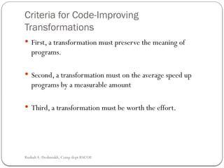
Criteria for Code-Improving
Transformations
First, a transformation must preserve the meaning of
programs.
Second, a transformation must on the average speed up
programs by a measurable amount
Third, a transformation must be worth the effort.
Rushali A. Deshmukh, Comp dept RSCOE
3.
Principal Sources ofOptimization
Strength Reduction :
Replace an expensive operation by a cheaper one.
Suppose the integer expression 5*i appears in a tight loop.
1.Multiplication is relatively expensive.
2.One solution: Generate code for i+i+i+i+i instead.
3.Another solution:Treat the expression as if it were written
(4*i)+i and do the multiplication as a shift left of 2 bits.
Generate the code to shift the value of i and then add the
original value of i.
Rushali A. Deshmukh, Comp dept RSCOE
4.
Principal Sources ofOptimization
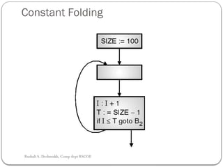
Constant folding :
Constant expressions are calculated during compilation.
Example 9.2
const NN = 4;
...
i:=2+NN; → i := 6
j:=i*5+a; → j := 30 + a
Rushali A. Deshmukh, Comp dept RSCOE
5.
Principal Sources ofOptimization
Constant propogation :
Many variables retain a constant value over a large portion of their lifetime,
compiler can note when a constant is assigned to variable and use that
constant instead of that variable.
Example 9.4
y=5
x=y
above code can be optimized as follows:
y = 5
.
.
x = 5
Rushali A. Deshmukh, Comp dept RSCOE
Principal Sources ofOptimization
Dead variable and dead code elimination
Dead code is a computer programming term for code in
the source code of a program, which is executed but whose
result is never used in any other computation.
The execution of dead code wastes computation time as its
results are never used.
Example
int f (int x, int y)
{
int z=x+y;
return x*y;
}
Rushali A. Deshmukh, Comp dept RSCOE
8.
Principal Sources ofOptimization
Common subexpression elimination
An occurrence of an expression E is called a common subexpression,if E was
previously computed and the values of variables in E have not changed since
the previous computation.
We can avoid recomputing the expression if we can use the previously
computed value.
Example
a = b * c + g;
d = b * c * d;
It may be worth (ie, program executes faster) transforming the code so that it is
translated as if it had been written:
tmp = b * c;
a = tmp + g;
d = tmp * d;
Rushali A. Deshmukh, Comp dept RSCOE
9.
Principal Sources ofOptimization
Copy propogation
From the following code:
y = x
z = 3 + y
Copy propagation would yield:
z = 3 + x
Rushali A. Deshmukh, Comp dept RSCOE
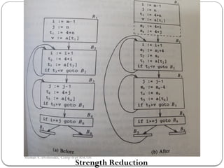
Loop unrolling
loopunrolling avoids a test at every iteration by recognizing that the number of iterations
is constant and replicating the body of the loop.
Suppose we have a loop like
begin
while I ≤ 100 do
begin
A[I] :=0;
I := I + 1;
end
end
We could do with 50 tests if we converted the code to
begin
while I ≤ 100 do
begin
A[I] :=0;
I := I + 1;
A[I] :=0;
I := I + 1;
end
end Rushali A. Deshmukh, Comp dept RSCOE
12.
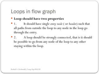
Loops in flowgraph
Loop should have two properties
1. It should have single entry node ( or header) such that
all paths from outside the loop to any node in the loop go
through the entry.
2. A loop should be strongly connected, that is it should
be possible to go from any node of the loop to any other
staying within the loop.
Rushali A. Deshmukh, Comp dept RSCOE
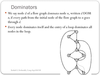
13.
Dominators
We saynode d of a flow graph dominates node n, written d DOM
n,if every path from the initial node of the flow graph to n goes
through d.
Every node dominates itself and the entry of a loop dom
inates all
nodes in the loop.
Rushali A. Deshmukh, Comp dept RSCOE
14.
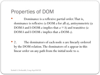
Properties of DOM
Dominance is a reflexive partial order.That is,
dominance is reflexive (a DOM a for all a), antisymmetric (a
DOM b and b DOM a implies that a = b) and transitive (a
DOM b and b DOM c implies that a DOM c).
2. The dominators of each node n are linearly ordered
by the DOM relation.The dominators of n appear in this
linear order on any path from the initial node to n.
Rushali A. Deshmukh, Comp dept RSCOE
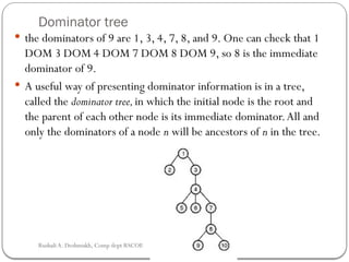
15.
Dominator tree
thedominators of 9 are 1, 3, 4, 7, 8, and 9. One can check that 1
DOM 3 DOM 4 DOM 7 DOM 8 DOM 9, so 8 is the immediate
dominator of 9.
A useful way of presenting dominator information is in a tree,
called the dominator tree,in which the initial node is the root and
the parent of each other node is its immediate dominator.All and
only the dominators of a node n will be ancestors of n in the tree.
Rushali A. Deshmukh, Comp dept RSCOE
16.
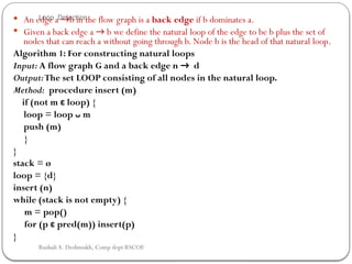
Loop Detection
Anedge a →b in the flow graph is a back edge if b dominates a.
Given a back edge a → b we define the natural loop of the edge to be b plus the set of
nodes that can reach a without going through b. Node b is the head of that natural loop.
Algorithm 1: For constructing natural loops
Input: A flow graph G and a back edge n → d
Output:The set LOOP consisting of all nodes in the natural loop.
Method: procedure insert (m)
if (not m ε loop) {
loop = loop ᴗ m
push (m)
}
}
stack = ø
loop = {d}
insert (n)
while (stack is not empty) {
m = pop()
for (p ε pred(m)) insert(p)
}
Rushali A. Deshmukh, Comp dept RSCOE
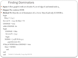
Finding Dominators
Input:A flow graph G with set of nodes N, set of edges E and initial node n0
Output:The realation DOM
Method:We D(n) the set of dominators of n. d is in D(n) if and only if d DOM n.
begin
D(n0) = { n0 }
for n in N – { n0} do D(n) = N
CHANGE = true
while CHANGE do
begin
CHANGE = false
for n in N –{ n0}
begin
NEWD = { n}U D ( p )
∩
p predecessor of n
if D(n) ≠ NEWD then CHANGE = true
D(n) = NEWD
end
end
end Rushali A. Deshmukh, Comp dept RSCOE
19.
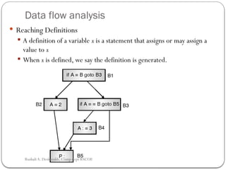
Data flow analysis
Reaching Definitions
A definition of a variable x is a statement that assigns or may assign a
value to x
When x is defined, we say the definition is generated.
Rushali A. Deshmukh, Comp dept RSCOE
20.
The first,which we call GEN[B] is the set of generated
definitions, those definitions within block B that reach the end
of the block.
The second set needed is KILL[B], which is the set of
definitions out
side of B that define identifiers that also have
definitions within B.
We can easily tell which identifiers have definitions within B
and we have already made a list of the definitions of each
identifier.
the set IN[B] consisting of all definitions reaching the point
just before the first statement of block B.
the set OUT[B] consisting of all definitions reaching the point
after the last statement of block B.
in[B] = out(P)
∪
out[B]=gen [B] (in [B] – kill[B])
∪
Rushali A. Deshmukh, Comp dept RSCOE
21.
Data Flow Equations
Each region (or NT) has four attributes:
gen[S]: Set of definitions generated by the block S.
If a definition d is in gen[S], then d reaches the end of block S.
kill[S]: Set of definitions killed by block S.
If d is in kill[S], d never reaches the end of block S. Every path from the
beginning of S to the end S must have a definition for a (where a is
defined by d).
22.
Data Flow Equations
in[S]:The set of definition those are live at the entry point of
block S.
out[S]:The set of definition those are live at the exit point of
block S.
The data flow equations are inductive or syntax directed.
gen and kill are synthesized attributes.
in is an inherited attribute.
23.
Data Flow Equations
gen[S] concerns with a single basic block. It is the set of
definitions in S that reaches the end of S.
In contrast out[S] is the set of definitions (possibly defined in
some other block) live at the end of S considering all paths
through S.
24.
Data Flow Equations
Singlestatement
d: a := b + c
[ ] [ ] ( [ ] [ ])
out S gen S in S kill S
Da: The set of definitions in the program for variable a
S
[ ] { }
[ ] { }
a
gen S d
kill S D d
25.
Data Flow Equations
Composition
S
S1
S2
21 2
2 1 2
[ ] [ ] ( [ ] [ ])
[ ] [ ] ( [ ] [ ])
gen S gen S gen S kill S
kill S kill S kill S gen S
1
2 1
2
[ ] [ ]
[ ] [ ]
[ ] [ ]
in S in S
in S out S
out S out S
26.
Data Flow Equations
if-then-else
S1S2
S
1 2
1 2
[ ] [ ] [ ]
[ ] [ ] [ ]
gen S gen S gen S
kill S kill S kill S
1
2
1 2
[ ] [ ]
[ ] [ ]
[ ] [ ] [ ]
in S in S
in S in S
out S out S out S
27.
Data Flow Equations
Loop
SS1
1
1
[ ] [ ]
[ ] [ ]
gen S gen S
kill S kill S
1 1
1
[ ] [ ] [ ]
[ ] [ ]
in S in S gen S
out S out S
28.
Data Flow Analysis
The attributes are computed for each region.The
equations can be solved in two phases:
gen and kill can be computed in a single pass of a basic block.
in and out are computed iteratively.
Initial condition for in for the whole program is
In can be computed top- down
Finally out is computed
29.
Iterative algorithm forReaching definitions
/* Initialize on the assumption in[B] = ø for all B *
change = true
for (each block B) out [B] = gen [B]
do {
change = false
for (each block B) {
NEWIN = out [P]
∪
P ε pred(B)
if (NEWIN ≠ in[B]){
change = true
in[B] = NEWIN
out[B] = gen [B] (in[B] – kill[B])
∪
}
}while (change)
Rushali A. Deshmukh, Comp dept RSCOE
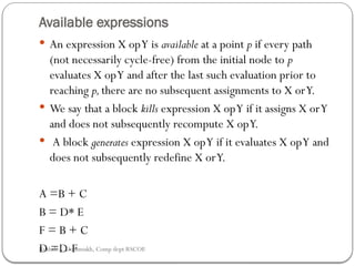
Available expressions
Anexpression X opY is available at a point p if every path
(not necessarily cycle-free) from the initial node to p
evaluates X opY and after the last such evaluation prior to
reaching p,there are no subsequent assignments to X orY.
We say that a block kills expres
sion X opY if it assigns X orY
and does not subsequently recompute X opY.
A block generates expression X opY if it evaluates X opY and
does not subsequently redefine X orY.
A =B + C
B = D* E
F = B + C
D =D-F
Rushali A. Deshmukh, Comp dept RSCOE
34.
Let Uis the “universal” set of all expressions appearing on the right
of one or more statements of the program.
out[n] be the same for the point following the end of n.
e_gen[n] to be the expressions generated by n and
e_kill[n] to be the set of expressions in U killed in n.
out[n] = in[n] - e_kill[n] U e_gen[n]
in[n] = ∩ out[p] for n not initial
where p is a predecessor of n
in[n0] = where n
Φ 0 is the initial node
Rushali A. Deshmukh, Comp dept RSCOE
35.
Global Common SubexpressionElimination
Algorithm
Begin
in[n1] = Φ
out[n1] = e_gen[n1]
/* in and out never change for the initial node, n1*/
for i = 2 to N do
begin
in[ni] = U
out[ni] = U – e_kill[ni]
end
Rushali A. Deshmukh, Comp dept RSCOE
36.
change = true
whilechange do
begin
change = false
for i = 2 to N do
begin
newin = ∩ out[p] p a predecessor of ni
if in[ni ] ≠ newin then
begin
in[ni] = newin
out[ni] = in[ni] - e_kill[ni] U e_gen[ni]
change = true
end
end
end
end
Rushali A. Deshmukh, Comp dept RSCOE
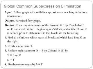
Global Common SubexpressionElimination
Input :A flow graph with available expression and reaching definitions
information.
Output : A revised flow graph.
Method : For every statement s of the formA := B op C such that B
op C is available at the beginning of s's block, and neither B nor C
is defined prior to statement s in that block, do the following:
1. Find all definitions which reach s's block and which have B op C on
the right.
2. Create a new nameT.
3. Replace each statement D = B op C found in (1) by
T = B op C
D =T
4. Replace statement s by A =T
Rushali A. Deshmukh, Comp dept RSCOE
39.
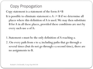
Copy Propogation
Copy statementis a statement of the form A=B
It is possible to eliminate statement s:A := B if we determine all
places where this definition of A is used.We may then substitute
B for A in all these places, provided these conditions are met by
every such use u ofA:
1.Statement s must be the only definition of A reaching u.
2. On every path from s to u,including paths that go through u
several times (but do not go through s a second time), there are
no assign
ments to B.
Rushali A. Deshmukh, Comp dept RSCOE
40.
in[n] isthe set of copiesA := B such that every path from the ini
tial
node to the beginning of n contains the statementA := B and subse
quent to the last occurrence of A := B, there are no assignments to B.
out[n] can be defined correspondingly but with respect to the end of n.
We say copy statement s:A := B is generated in block n if s occurs in n
and there is no subsequent assignment to B within n.
We say s:A := B is killed in n if A or B is assigned there and s is not in n.
Let U be the "universal" set of all copy statements in the program.
c_gen[n] to be the set of all copies generated in n.
c_kill[n] to be the set of copies in U which are killed in n.
out[n] = in[n] - c_kill[n] U c_gen[n]
in[n] = ∩ out[p] for n not initial p a predecessor of n
in[n0] = where n
Φ 0 is the initial node
Rushali A. Deshmukh, Comp dept RSCOE
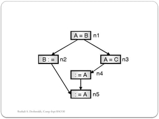
c_gen[n1] ={A = B}
c_gen[n3] = {A = C}
c_kill[n2] = {A = B} since B is assigned in n2
c_kill[n1] = {A = C} sinceA is assigned in n1
c_kill[n3] = {A = B}
other c_gen’s and c_kill’s are Φ
in[n1] = Φ
one pass determines that in[n2] = in[n3] = out[n1] = {A = B}
out[n2] = Φ
out[n3] = in[n4] = out[n4] = {A = C}
in[n5] = out[n2] Ç out[n4] = Φ
We observe that neitherA = B norA=C reaches the use of A in n5
Rushali A. Deshmukh, Comp dept RSCOE
43.
Algorithm Copy propagation
Input : A flow graph with ud-chaining information represented by sets
r_in[n] giving the definitions reaching node n and with c_in[n] representing
the solution to
that is the set of copies A := B that reach node n along every path,
with no assignment to A or B following the last occurrence of A : = B on
the path.
Output : A revised flow graph.
Method : For each copy s:A := B do the following.
Determine those uses of A which are reached by the definition of A, namely,
s:A := B.
Determine whether for every use of A found in (1), s is in c_in[n], where n is
the block of this particular use and moreover no definitions ofA or B occur
prior to this use of A within n.
3. If s meets the conditions of (2), then remove s and replace all uses of
A found in (1) by B.
Rushali A. Deshmukh, Comp dept RSCOE
Live Variables
Here wewish to know for name A and point p whether the value, of
A at p could be used along some path in the flow graph starting at
p.If so, we say A is live at p otherwise A is dead at p.
Use of live variable information :
Another more important use for live variable information comes
when we generate object code.
After a value is computed in a register and presumably used within
a block, it is not necessary to store that value if it is dead at the end
of the block.
Also, if all registers are full and we need another register, we
should favor using a register with a dead value since that value does
not have to be stored.
Rushali A. Deshmukh, Comp dept RSCOE
46.
Dataflow forliveness :
Using the sets use [B] and def [B]
def [B] is the set of variables assigned values in B prior to any use of
that varible in B.
Use [B] is the set of variables whose values may be used in B prior to
any definition of the variable.
A variable comes live into a block (in in[B]), if it is either used before
redefinition of it is live coming out of the block and is not redefined in
the block.
A variable comes live into a block (in out[B]), ifand only if it is live
coming into one of its successors.
Dataflow equations for liveness :
in [B] = use[B] (out [B] – def [B])
∪
out[B] = in[S]
∪
Rushali A. Deshmukh, Comp dept RSCOE
47.
Example: Liveness
r1 =r2 + r3
r6 = r4 – r5
r4 = 4
r6 = 8
r6 = r2 + r3
r7 = r4 – r5
r2, r3, r4, r5 are all live as they
are consumed later, r6 is dead
as it is redefined later
r4 is dead, as it is redefined.
So is r6. r2, r3, r5 are live
What does this mean?
r6 = r4 – r5 is useless,
it produces a dead value !!
Get rid of it!
48.
Live variable analysis
Input : A flow graph with def and use computed for each block.
Output : out[B], the set of variables live on exit from each block B
of the flow graph
Begin
For each block B do in[B] = Φ
While changes to any of the in’s occur do
For each block B do
begin
out[B] = U in[S]
S a successor of B
in[B] = use[B] U ( out[B] – def[B])
end
end
Rushali A. Deshmukh, Comp dept RSCOE
49.
DU/UD Chains
Convenientway to access/use reaching definition information.
Def-Use chains (DU chains)
Given a def, what are all the possible consumers of the definition
produced
Use-Def chains (UD chains)
Given a use, what are all the possible producers of the definition
consumed
Rushali A. Deshmukh,Comp dept RSCOE
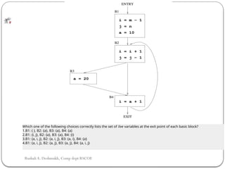
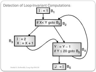
Which one of the following choices correctly lists the set of live variables at the exit point of each basic block?
1.B1: { }, B2: {a}, B3: {a}, B4: {a}
2.B1: {i, j}, B2: {a}, B3: {a}, B4: {i}
3.B1: {a, i, j}, B2: {a, i, j}, B3: {a, i}, B4: {a}
4.B1: {a, i, j}, B2: {a, j}, B3: {a, j}, B4: {a, i, j}
Constant folding
Input: A flow graph with ud-chaining information computed .
Output : A revised flow graph
while changes occur do
for all statements s of the program do
begin
for each operand B of s do
if there is a unique definition of B that reaches s and that definition is of the
form B: = c for a constant c
then replace B by c in s;
if all operands of s are now constants then
begin
evaluate the right side of s;
replace s byA : = e,whereA is the name assigned to by s and e is the value of
the right side of s
end
end
Rushali A. Deshmukh, Comp dept RSCOE
54.
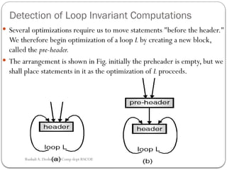
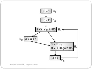
Detection of LoopInvariant Computations
Several optimizations require us to move statements "before the header."
We therefore begin optimization of a loop L by creating a new block,
called the pre-header.
The arrangement is shown in Fig. initially the preheader is empty, but we
shall place statements in it as the optimization of L proceeds.
Rushali A. Deshmukh, Comp dept RSCOE
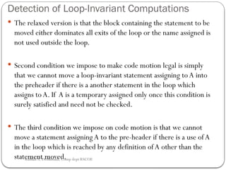
Detection of Loop-InvariantComputations
The relaxed version is that the block containing the statement to be
moved either dominates all exits of the loop or the name assigned is
not used outside the loop.
Second condition we impose to make code motion legal is simply
that we cannot move a loop-invariant statement assigning toA into
the preheader if there is a another statement in the loop which
assigns toA. If A is a temporary assigned only once this condition is
surely satisfied and need not be checked.
The third condition we impose on code motion is that we cannot
move a statement assigning A to the pre-header if there is a use ofA
in the loop which is reached by any definition of A other than the
statement moved.
Rushali A. Deshmukh, Comp dept RSCOE
58.
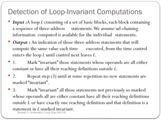
Detection of Loop-InvariantComputations
Input :A loop L consisting of a set of basic blocks, each block containing
a sequence of three-address statements.We assume ud-chaining
information computed is available for the individual statements.
Output : An indication of those three-address statements that will
compute the same value each time executed, from the time control
enters the loop L until control next leaves L.
1. Mark “invariant” those statements whose operands are all either
con
stant or have all their reaching definitions outside L.
2. Repeat step (3) until at some repetition no new statements are
marked “invariant”.
3. Mark “invariant” all those statements not previously so marked
whose operands all are either constant have all their reaching definitions
out
side L or have exactly one reaching definition and that definition is a
statement in L marked invariant.
Rushali A. Deshmukh, Comp dept RSCOE
59.
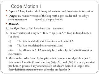
Code Motion I
Input : A loop L with ud-chaining information and dominator information.
Output :A revised version of the loop with a pre-header and (possibly)
some statements moved to the pre-header.
Method :
1. Use Algorithm to find loop-invariant statements.
2. For each statement s, sayA = B,A = op B, orA = B op C, found in step
(1) check
(i) That it is in a block which dominates all exits of L.
(ii) That A is not defined elsewhere in L and
(iii) That all uses in L of A can only be reached by the definition of A in
statement s.
3. Move in the order found by loop invariant computation algorithm , each
statement s found in (1) and meeting (2i), (2ii), and (2iii) to a newly created
pre-header, provided any operands of s which are defined in loop L have
their definition statements moved to the pre-header D.
Rushali A. Deshmukh, Comp dept RSCOE
60.
Code Motion II
Input : A loop L with ud-chaining information, dominator information and information as
to which identifiers are live immediately after each loop exit.
Output :A revised version of the loop with a pre-header and (possibly) more
statements moved to the pre-header.
Method :
1. Use Algorithm to find loop-invariant statements.
2. For each-statement S found in (1) check that it either
a) Meets the three conditions of step (2) of code motion I Algorithm or
b) Defines a name which is not live on entry to any successor of any exit of L
if that successor is not in I and which meets conditions (ii) and (iii) of step (2) of code
motion I Algorithm .That is, we relax the condition that statement 5 appears in a block
that dominates all exits of L.
3. Move in the order found by loop invariant computation algorithm , each statement
s found in (1) and satisfying the criterion of step (2) to the pre-header, pro
vided any
operands of s which are defined in L also have their definitions moved to the pre-header D.
Rushali A. Deshmukh, Comp dept RSCOE
61.
Elimination of InductionVariables
A variable x is called an induction variable of a loop L if every time the
variable x changes values, it is incremented or decremented by some
constant.
A basic induction variable i is a variable that only has assignments of the
form i = i ± c
Associated with each induction variable j is a triple (i,c,d) where i is a basic
induction variable and c and d are constants such that j = c * i + d.
In this case j belongs to the family of i
The basic induction variable i belongs to its own family with the associated
triple (i,1,0).
Rushali A. Deshmukh, Comp dept RSCOE
62.
Detection of inductionvariables
Input :A loop L with reaching definition information and loop-invariant computation
information.
Output :A set of induction variables.Associated with each induction variable j is a triple
(i,c,d) where i is a basic induction variable and c and d are constants such that
j = c * i + d. In this case j belongs to the family of i.
The basic induction variable i belongs to its own family.
Method :
1. Find all basic induction variables in the loop L.Associated with each basic induction
variable i is the triple (i,1,0).
2. Find variables k with a single assignment in the loop with one of the following forms:
k = j * b, k = b * j, k = j/b, k = j ± b, k = b ± j, where
b is a constant and j is an induction variable.
3. If j is not basic and in the family of i then there must be.
No assignment of i between the assignment of j and k.
No definition of j outside the loop that reaches k.
Rushali A. Deshmukh, Comp dept RSCOE
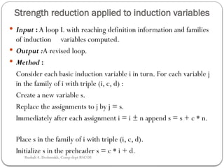
Strength reduction appliedto induction variables
Input : A loop L with reaching definition information and families
of induction variables computed.
Output :A revised loop.
Method :
Consider each basic induction variable i in turn. For each variable j
in the family of i with triple (i, c, d) :
Create a new variable s.
Replace the assignments to j by j = s.
Immediately after each assignment i = i ± n append s = s + c * n.
Place s in the family of i with triple (i, c, d).
Initialize s in the preheader s = c * i + d.
Rushali A. Deshmukh, Comp dept RSCOE
65.
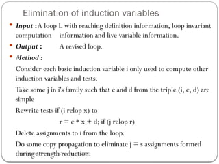
Elimination of inductionvariables
Input :A loop L with reaching definition information, loop invariant
computation information and live variable information.
Output : A revised loop.
Method :
Consider each basic induction variable i only used to compute other
induction variables and tests.
Take some j in i's family such that c and d from the triple (i, c, d) are
simple
Rewrite tests if (i relop x) to
r = c * x + d; if (j relop r)
Delete assignments to i from the loop.
Do some copy propagation to eliminate j = s assignments formed
during strength reduction.
Rushali A. Deshmukh, Comp dept RSCOE
66.
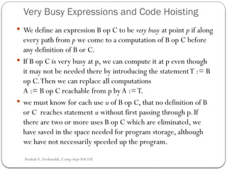
Very Busy Expressionsand Code Hoisting
We define an expression B op C to be very busy at point p if along
every path from p we come to a computation of B op C before
any definition of B or C.
If B op C is very busy at p, we can compute it at p even though
it may not be needed there by introducing the statementT := B
op C.Then we can replace all computations
A := B op C reachable from p by A :=T.
we must know for each use u of B op C, that no definition of B
or C reaches statement u without first passing through p.If
there are two or more uses B op C which are eliminated, we
have saved in the space needed for program storage, although
we have not necessarily speeded up the program.
Rushali A. Deshmukh, Comp dept RSCOE
![Loop unrolling
loop unrolling avoids a test at every iteration by recognizing that the number of iterations
is constant and replicating the body of the loop.
Suppose we have a loop like
begin
while I ≤ 100 do
begin
A[I] :=0;
I := I + 1;
end
end
We could do with 50 tests if we converted the code to
begin
while I ≤ 100 do
begin
A[I] :=0;
I := I + 1;
A[I] :=0;
I := I + 1;
end
end Rushali A. Deshmukh, Comp dept RSCOE](https://image.slidesharecdn.com/compilerdesigncodeoptimization-250505081416-d3095962/85/Compiler-Design_Code-Optimization-tech-pptx-11-320.jpg)
![ The first, which we call GEN[B] is the set of generated
definitions, those definitions within block B that reach the end
of the block.
The second set needed is KILL[B], which is the set of
definitions out
side of B that define identifiers that also have
definitions within B.
We can easily tell which identifiers have definitions within B
and we have already made a list of the definitions of each
identifier.
the set IN[B] consisting of all definitions reaching the point
just before the first statement of block B.
the set OUT[B] consisting of all definitions reaching the point
after the last statement of block B.
in[B] = out(P)
∪
out[B]=gen [B] (in [B] – kill[B])
∪
Rushali A. Deshmukh, Comp dept RSCOE](https://image.slidesharecdn.com/compilerdesigncodeoptimization-250505081416-d3095962/85/Compiler-Design_Code-Optimization-tech-pptx-20-320.jpg)
![Data Flow Equations
Each region (or NT) has four attributes:
gen[S]: Set of definitions generated by the block S.
If a definition d is in gen[S], then d reaches the end of block S.
kill[S]: Set of definitions killed by block S.
If d is in kill[S], d never reaches the end of block S. Every path from the
beginning of S to the end S must have a definition for a (where a is
defined by d).](https://image.slidesharecdn.com/compilerdesigncodeoptimization-250505081416-d3095962/85/Compiler-Design_Code-Optimization-tech-pptx-21-320.jpg)
![Data Flow Equations
in[S]:The set of definition those are live at the entry point of
block S.
out[S]:The set of definition those are live at the exit point of
block S.
The data flow equations are inductive or syntax directed.
gen and kill are synthesized attributes.
in is an inherited attribute.](https://image.slidesharecdn.com/compilerdesigncodeoptimization-250505081416-d3095962/85/Compiler-Design_Code-Optimization-tech-pptx-22-320.jpg)
![Data Flow Equations
gen[S] concerns with a single basic block. It is the set of
definitions in S that reaches the end of S.
In contrast out[S] is the set of definitions (possibly defined in
some other block) live at the end of S considering all paths
through S.](https://image.slidesharecdn.com/compilerdesigncodeoptimization-250505081416-d3095962/85/Compiler-Design_Code-Optimization-tech-pptx-23-320.jpg)
![Data Flow Equations
Single statement
d: a := b + c
[ ] [ ] ( [ ] [ ])
out S gen S in S kill S
Da: The set of definitions in the program for variable a
S
[ ] { }
[ ] { }
a
gen S d
kill S D d
](https://image.slidesharecdn.com/compilerdesigncodeoptimization-250505081416-d3095962/85/Compiler-Design_Code-Optimization-tech-pptx-24-320.jpg)
![Data Flow Equations
Composition
S
S1
S2
2 1 2
2 1 2
[ ] [ ] ( [ ] [ ])
[ ] [ ] ( [ ] [ ])
gen S gen S gen S kill S
kill S kill S kill S gen S
1
2 1
2
[ ] [ ]
[ ] [ ]
[ ] [ ]
in S in S
in S out S
out S out S
](https://image.slidesharecdn.com/compilerdesigncodeoptimization-250505081416-d3095962/85/Compiler-Design_Code-Optimization-tech-pptx-25-320.jpg)
![Data Flow Equations
if-then-else
S1 S2
S
1 2
1 2
[ ] [ ] [ ]
[ ] [ ] [ ]
gen S gen S gen S
kill S kill S kill S
1
2
1 2
[ ] [ ]
[ ] [ ]
[ ] [ ] [ ]
in S in S
in S in S
out S out S out S
](https://image.slidesharecdn.com/compilerdesigncodeoptimization-250505081416-d3095962/85/Compiler-Design_Code-Optimization-tech-pptx-26-320.jpg)
![Data Flow Equations
Loop
S S1
1
1
[ ] [ ]
[ ] [ ]
gen S gen S
kill S kill S
1 1
1
[ ] [ ] [ ]
[ ] [ ]
in S in S gen S
out S out S
](https://image.slidesharecdn.com/compilerdesigncodeoptimization-250505081416-d3095962/85/Compiler-Design_Code-Optimization-tech-pptx-27-320.jpg)
![Iterative algorithm for Reaching definitions
/* Initialize on the assumption in[B] = ø for all B *
change = true
for (each block B) out [B] = gen [B]
do {
change = false
for (each block B) {
NEWIN = out [P]
∪
P ε pred(B)
if (NEWIN ≠ in[B]){
change = true
in[B] = NEWIN
out[B] = gen [B] (in[B] – kill[B])
∪
}
}while (change)
Rushali A. Deshmukh, Comp dept RSCOE](https://image.slidesharecdn.com/compilerdesigncodeoptimization-250505081416-d3095962/85/Compiler-Design_Code-Optimization-tech-pptx-29-320.jpg)
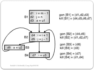
![Block
B
gen[B] Bit vector kill[b] Bit vector
B1 {d1,d2,d3} 1110000 {d4,d5,d6,d7} 0001111
B2 { d4,d5} 0001100 {d1, d2, d7} 1100001
B3 { d6} 0000010 { d3} 0010000
B4 { d7} 0000001 { d1, d4} 1001000
in[B2] = out[B1] È out [B3] È out [B4]
= 111 0000 + 000 0010 + 000 0001 = 11
0011
Out[B2] = gen[B2] È (in[B2] – kill [B2])
= 000 1100 + ( 111 0011 – 110 0001) = 00
1110
Rushali A. Deshmukh, Comp dept RSCOE](https://image.slidesharecdn.com/compilerdesigncodeoptimization-250505081416-d3095962/85/Compiler-Design_Code-Optimization-tech-pptx-31-320.jpg)
![Block Inital Pass1 Pass2
in[B] out[B] in[B] out[B] in[B] out[B]
B1 000 0000 111 0000 000 0000 111 0000 000 0000 111 0000
B2 000 0000 000 1 100 111 0011 001 1110 111 1111 001 1110
B3 000 0000 000 0010 001 1110 000 1110 001 1110 000 1110
B4 000 0000 000 0001 001 1110 001 0111 001 1110 001 0111
Rushali A. Deshmukh, Comp dept RSCOE](https://image.slidesharecdn.com/compilerdesigncodeoptimization-250505081416-d3095962/85/Compiler-Design_Code-Optimization-tech-pptx-32-320.jpg)
![ Let U is the “universal” set of all expressions appearing on the right
of one or more statements of the program.
out[n] be the same for the point following the end of n.
e_gen[n] to be the expressions generated by n and
e_kill[n] to be the set of expressions in U killed in n.
out[n] = in[n] - e_kill[n] U e_gen[n]
in[n] = ∩ out[p] for n not initial
where p is a predecessor of n
in[n0] = where n
Φ 0 is the initial node
Rushali A. Deshmukh, Comp dept RSCOE](https://image.slidesharecdn.com/compilerdesigncodeoptimization-250505081416-d3095962/85/Compiler-Design_Code-Optimization-tech-pptx-34-320.jpg)
![Global Common Subexpression Elimination
Algorithm
Begin
in[n1] = Φ
out[n1] = e_gen[n1]
/* in and out never change for the initial node, n1*/
for i = 2 to N do
begin
in[ni] = U
out[ni] = U – e_kill[ni]
end
Rushali A. Deshmukh, Comp dept RSCOE](https://image.slidesharecdn.com/compilerdesigncodeoptimization-250505081416-d3095962/85/Compiler-Design_Code-Optimization-tech-pptx-35-320.jpg)
![change = true
while change do
begin
change = false
for i = 2 to N do
begin
newin = ∩ out[p] p a predecessor of ni
if in[ni ] ≠ newin then
begin
in[ni] = newin
out[ni] = in[ni] - e_kill[ni] U e_gen[ni]
change = true
end
end
end
end
Rushali A. Deshmukh, Comp dept RSCOE](https://image.slidesharecdn.com/compilerdesigncodeoptimization-250505081416-d3095962/85/Compiler-Design_Code-Optimization-tech-pptx-36-320.jpg)
![ in[n] is the set of copiesA := B such that every path from the ini
tial
node to the beginning of n contains the statementA := B and subse
quent to the last occurrence of A := B, there are no assignments to B.
out[n] can be defined correspondingly but with respect to the end of n.
We say copy statement s:A := B is generated in block n if s occurs in n
and there is no subsequent assignment to B within n.
We say s:A := B is killed in n if A or B is assigned there and s is not in n.
Let U be the "universal" set of all copy statements in the program.
c_gen[n] to be the set of all copies generated in n.
c_kill[n] to be the set of copies in U which are killed in n.
out[n] = in[n] - c_kill[n] U c_gen[n]
in[n] = ∩ out[p] for n not initial p a predecessor of n
in[n0] = where n
Φ 0 is the initial node
Rushali A. Deshmukh, Comp dept RSCOE](https://image.slidesharecdn.com/compilerdesigncodeoptimization-250505081416-d3095962/85/Compiler-Design_Code-Optimization-tech-pptx-40-320.jpg)
![ c_gen[n1] = {A = B}
c_gen[n3] = {A = C}
c_kill[n2] = {A = B} since B is assigned in n2
c_kill[n1] = {A = C} sinceA is assigned in n1
c_kill[n3] = {A = B}
other c_gen’s and c_kill’s are Φ
in[n1] = Φ
one pass determines that in[n2] = in[n3] = out[n1] = {A = B}
out[n2] = Φ
out[n3] = in[n4] = out[n4] = {A = C}
in[n5] = out[n2] Ç out[n4] = Φ
We observe that neitherA = B norA=C reaches the use of A in n5
Rushali A. Deshmukh, Comp dept RSCOE](https://image.slidesharecdn.com/compilerdesigncodeoptimization-250505081416-d3095962/85/Compiler-Design_Code-Optimization-tech-pptx-42-320.jpg)
![Algorithm Copy propagation
Input : A flow graph with ud-chaining information represented by sets
r_in[n] giving the definitions reaching node n and with c_in[n] representing
the solution to
that is the set of copies A := B that reach node n along every path,
with no assignment to A or B following the last occurrence of A : = B on
the path.
Output : A revised flow graph.
Method : For each copy s:A := B do the following.
Determine those uses of A which are reached by the definition of A, namely,
s:A := B.
Determine whether for every use of A found in (1), s is in c_in[n], where n is
the block of this particular use and moreover no definitions ofA or B occur
prior to this use of A within n.
3. If s meets the conditions of (2), then remove s and replace all uses of
A found in (1) by B.
Rushali A. Deshmukh, Comp dept RSCOE](https://image.slidesharecdn.com/compilerdesigncodeoptimization-250505081416-d3095962/85/Compiler-Design_Code-Optimization-tech-pptx-43-320.jpg)
![ Dataflow for liveness :
Using the sets use [B] and def [B]
def [B] is the set of variables assigned values in B prior to any use of
that varible in B.
Use [B] is the set of variables whose values may be used in B prior to
any definition of the variable.
A variable comes live into a block (in in[B]), if it is either used before
redefinition of it is live coming out of the block and is not redefined in
the block.
A variable comes live into a block (in out[B]), ifand only if it is live
coming into one of its successors.
Dataflow equations for liveness :
in [B] = use[B] (out [B] – def [B])
∪
out[B] = in[S]
∪
Rushali A. Deshmukh, Comp dept RSCOE](https://image.slidesharecdn.com/compilerdesigncodeoptimization-250505081416-d3095962/85/Compiler-Design_Code-Optimization-tech-pptx-46-320.jpg)

![Live variable analysis
Input : A flow graph with def and use computed for each block.
Output : out[B], the set of variables live on exit from each block B
of the flow graph
Begin
For each block B do in[B] = Φ
While changes to any of the in’s occur do
For each block B do
begin
out[B] = U in[S]
S a successor of B
in[B] = use[B] U ( out[B] – def[B])
end
end
Rushali A. Deshmukh, Comp dept RSCOE](https://image.slidesharecdn.com/compilerdesigncodeoptimization-250505081416-d3095962/85/Compiler-Design_Code-Optimization-tech-pptx-48-320.jpg)
![Example: DU/UD Chains
1: r1 = MEM[r2+0]
2: r2 = r2 + 1
3: r3 = r1 * r4
4: r1 = r1 + 5
5: r3 = r5 – r1
6: r7 = r3 * 2
7: r7 = r6
8: r2 = 0
9: r7 = r7 + 1
10: r8 = r7 + 5
11: r1 = r3 – r8
12: r3 = r1 * 2
DU Chain of r1:
(1) -> 3,4
(4) ->5
DU Chain of r3:
(3) -> 11
(5) -> 11
(12) ->
UD Chain of r1:
(12) -> 11
UD Chain of r7:
(10) -> 6,9](https://image.slidesharecdn.com/compilerdesigncodeoptimization-250505081416-d3095962/85/Compiler-Design_Code-Optimization-tech-pptx-50-320.jpg)