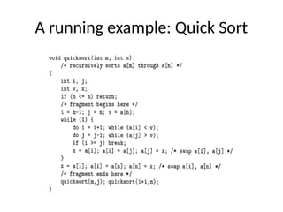
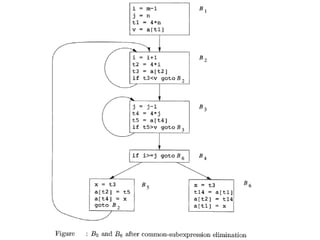
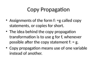
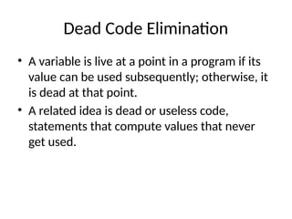
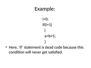
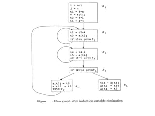
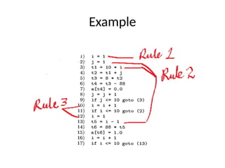
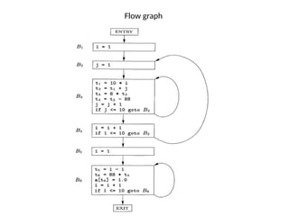
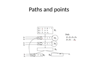
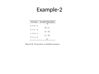
The document discusses machine-independent optimization techniques in programming, focusing on code improvement through local and global optimizations, including eliminating unnecessary instructions and applying transformations like copy propagation and dead code elimination. It introduces data flow analysis and the use of flow graphs to represent control structures and optimize code execution paths. Key concepts like reaching definitions, live variable analysis, and available expressions are illustrated with examples to demonstrate their importance in enhancing program efficiency.

1. Unit-5
Machine Independent
Optimization

2. INTRODUCTION
• Elimination of unnecessary instructions in object code or
the replacement of one sequence of instructions by a
faster sequence of instructions that does the same thing
is called as code improvement or code optimization.
• Local Code Optimization is the done improvement within
the basic block.
• Global code optimization improvemnets happens across
basic blocks.
• Most global optimizations are based on data flow
analyses.(which gathers information about a program)

3. Principal Sources Of Optimization
• A compiler optimization must preserve the
semantics of the original program.
• Causes of Redundancy:
• It is the side effect of having written the
program in a high level language.
• As a program is compiled each of these high
level data structure accesses expands into
number of low level operations.

4. A running example: Quick Sort

5. Three Address Code

6. Flow Graph of Quick
Sort

7. Local Common Subexpression

8. Global Common Subexpression
• An occurrence of an expression E is called a
Common subexpression if E was Previously
computed and the values of the variables in E
have not changed since the previous
Computation

10. Copy Propagation
• Assignments of the form f: =g called copy
statements, or copies for short.
• The idea behind the copy propagation
transformation is to use g for f, whenever
possible after the copy statement f: = g.
• Copy propagation means use of one variable
instead of another.

11. Example
• For example:
• x=Pi;
• ……
• A=x*r* r;
• The optimization using copy propagation can
be done as follows: A=Pi*r*r;
• Here the variable x is eliminated

12. Dead Code Elimination
• A variable is live at a point in a program if its
value can be used subsequently; otherwise, it
is dead at that point.
• A related idea is dead or useless code,
statements that compute values that never
get used.

13. Example:
i=0;
if(i=1)
{
a=b+5;
}
• Here, ‘if’ statement is dead code because this
condition will never get satisfied.

14. Code Motion
• Loops are most important place for optimizations especially
the inner loops.They spend the bulk of their time.
• The running time of a program may be improved if we
decrease the number of instructions in an inner loop.
• An important modification that decreases the amount of
code in a loop is code motion.
• The transformation that takes an expression that yields the
same result independent of number of times a loop is
executed is a loop-invariant computation.

15. Example

16. Induction variables and reduction in strength
• A variable x is said to be an induction variable if
there is a positive or negative constant c such
that each time x is assigned value increases by c.
• i and t2 are induction variables
in a loop containing B2
• When there are two or more induction variables
in a loop, it may be possible to get rid of all but
one, by the process of induction-variable
elimination

17. Strength Reduction
• Reduction in strength replaces expensive operations
by equivalent cheaper ones on the target machine.
• For example, x² is invariably cheaper to implement
as x*x than as a call to an exponentiation routine.
• Fixed-point multiplication or division by a power of
two is cheaper to implement as a shift.
• Floating-point division by a constant can be
implemented as multiplication by a constant, which
may be cheaper.

20. Introduction to Data-Flow Analysis
• Data Flow analysis refers to a body of technique
that derive information about the flow of data
along the program execution path.
• To achieve global optimization
• Example: we need to determine two textually
identical expressions evaluate to the same value
along the execution path
• An result of assignment is not used along any
subsequent execution path

21. Flow Graphs
• Graph representation of intermediate code that helps
in discussing code generation.
• Representation:
a) Partition the intermediate code into basic blocks
1) flow of control can enter the basic block through
the first instruction in the block
2) Control will leave block without halting or
branching
b) The basic blocks becomes the nodes of the flow graph

22. Basic blocks
• First basic block is formed with first instruction
and keep adding instructions until if we meet
either a jump or conditional jump or a label
on following instruction else keep on adding
the instructions into the block.
• Then we try to find out the leaders and break
and create the blocks

23. Algorithm to find blocks
• First we detemine the instructions in the
intermediate code thatare leaders
• The rules for finding the leaders
• 1) The first three address instructions in the
intermediate code is a leader
• 2) any instruction that is the target of a
conditional or unconditional jump is a leader.
• 3) Any instruction that immediately follows a
conditional or unconditional jump is a leader.

24. Example

25. Flow graph

26. Flow Graphs
• Once the intermediate code is parttitioned
into basic blocks,we represent the flow of
control between them by a flow graph
• The nodes of the flow graph are a basic blocks.
• There is an edge from block B to block C if and
only if

27. • We say that B is a predecessor of C and C is a
successor of B.
• We add entry and exit which is not part of
intermediate instructions.

28. Data Flow Abstraction
• The execution of a program can be viewed as a series
of transformations of the program state which
consists of the values of all the variables in the
program,stack frames.
• Each execution of an intermediate code statement
transforms an input state to output state.
• The input state is associated with the program point
before the statement and the output state is
associated with the program point after the
statement.

29. • To analyze the behavior of a program we must
consider all the possible sequences of
program points(“paths”) through a flow graph
that the program execution can take.
• Then from possible program states at each
point the information we need will be used as
a solution for solving a data flow analysis
problem.

30. Possible execution paths
• Within one basic block,the program point
after a statement is the same as the program
point before the next statement.
• If there is an edge from block B1 to Block B2
then the program point after the last
statement of B1 may be followed
immediatedly by the program point before the
first statement of B2.

31. • Thus we define execution paths from point
p1,p2,…….pn to be a sequence of points
p1,p2,p3……pn such hat for each i=1,2,3…..n-1
• 1) pi is the point immediatedly preceding a
statement and pi+1 is the point after the same
statement.
• 2) pi is the end of the some block and pi+1 is the
beginning of a successor block.

32. Paths and points

33. Data Flow analysis schema
• Every program point is associated with the data flow value that
represents the abstraction of the set of all possible program
states that can be observed for that point.
• The set of all possible data flow values is the domain for this
application.
• We can denote the data flow values before and after each
statement s by IN[s] and OUT[s].
• The data flow problem is to find a solution to set of constraints:
• 1) those based on semantics of he statements(transfer
functions)
• 2) based on flow of control

34. Transfer Functions

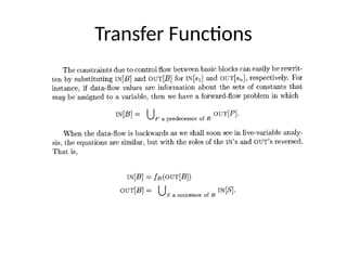
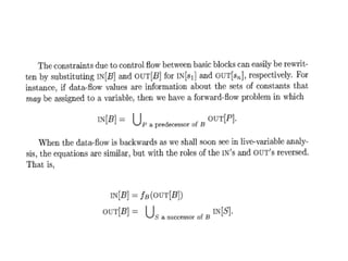
35. Control Flow Constraints
• The second set of constraints on data-flow
values is derived from the flow of control.
Within a basic block, control flow is simple. If a
block B consists of statements S1,S2…..Sn in
that order, then the control-flow value out of
Si; is the same as the control-flow value into
Si+1. That is,
IN[Si+1] = OUT[Si] for all = 1,2,.

36. DATA FLOW SCHEMES ON BASIC BLOCKS
• Control flows from the beginning to the end of the block,
without interruption or branching.
• Thus, we can restate the schema in terms of data-flow
values entering and leaving the blocks.
• We denote the data-flow values immediately before and
immediately after each basic block B by IN[B] and OUT[B],
respectively.
• The constraints involving IN[B] and OUT[B] can be derived
from those involving IN[s] and OUT[s] for the various
statements, sin B as follows.

38. REACHING DEFINTIONS

39. • A definition d reaches a point p
– if there is a path from the point immediately
following d to p and
– d is not killed along the path (i.e. there is not
redefinition of the same variable in the path)
• A definition of a variable is killed between two
points when there is another definition of that
variable along the path.

43. Iterative Algorithm to compute reaching definitions
Reaching Definitions are defined
by equations:

45. Example

48. Live Variable analysis
• In live variable analysis we know for variable x
and point p whether the value of x at p could
be used along some path in the flow graph
starting at p.if so we say x is live at p
otherwise x is dead at p.
• Important use
• Register allocation

49. We first define the transfer functions of individual
statements and then we compute IN[B] and
OUT[B].

53. Iterative algorithm to compute live variables

54. Available Expressions
• An expression x+y is available at a,point p if every
path from the entry node to p evaluates x+y and
after the last such evaluation prior to reaching p,
there are no subsequent assignments to x or y.
• We say that a block kills expression x+y if it
assigns x or y and does not subsequent
recompute x+y.
• A block generates expression x+y if it defnetly
evaluates x+y and does not define x+y.

55. Example

56. Example 2

57. • The following equations relate the unknoowns
IN and OUT to each other and the kown
quantities e_gen and e_kill.

58. Iterative Algorithm

59. Available Expression
• An Expression x+y is available at a point p if
every path from the entry node to p evaluates
x+y and after the last such evaluation prior to
reaching p, there are no subsequent
assignments to x or y.
• The Primary buse of available expression
information is for detecting global common
subexpressions.

60. Example
In Fig(a) the expression 4*I in block B3 will be common subexpression
if 4*I is available at the entry point of block B3.It will be available if I is
not assigned a new value in block B2.
In Fig(b) 4*I is recomputed after I is assigned in B2.

61. Example-2

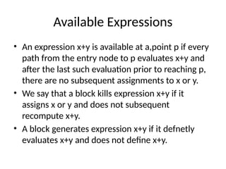
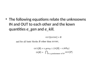
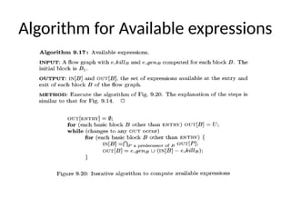
62. • For each block B, let IN{B] be the set of expressions in U
that are available at the point just before the beginning
of B.
• Let OUT[B] be the same for the point following the end
of B.
• Define e.gens to be the expressions generated by B and
e.killp to be the set of expressions in U killed in B.
• Note that IN, OUT, e-gen, and kill can all be represented
by bit vectors.
• The following equations relate the unknowns IN and OUT
to each other and the known quantities egen and e kill:

64. Algorithm for Available expressions