This document describes a narrow band region approach for 2D and 3D image segmentation using deformable curves and surfaces. Specifically, it develops a region energy term involving a fixed-width band around the evolving curve or surface. This energy achieves a balance between local gradient features and global region statistics. The region energy is formulated to allow efficient computation on explicit parametric models and implicit level set models. Two different region terms are introduced, each suited to different configurations of the target object and its surroundings. The document derives the mathematical framework for computing the region energies and their gradients to allow minimization via gradient descent. It then discusses numerical implementations and provides experiments segmenting medical and natural images.

1. Narrow band region-based active contours and surfaces for 2D and 3D segmentation
Julien Mille
Universit´ Fran¸ois Rabelais de Tours, Laboratoire Informatique (EA2101)
e c
64 avenue Jean Portalis, 37200 Tours, France
Abstract
We describe a narrow band region approach for deformable curves and surfaces in the perspective of 2D and 3D image
segmentation. Basically, we develop a region energy involving a fixed-width band around the curve or surface. Classical
region-based methods, like the Chan-Vese model, often make strong assumptions on the intensity distributions of the
searched object and background. In order to be less restrictive, our energy achieves a trade-off between local features
of gradient-like terms and global region features. Relying on the theory of parallel curves and surfaces, we perform a
mathematical derivation to express the region energy in a curvature-based form allowing efficient computation on explicit
models. We introduce two different region terms, each one being dedicated to a particular configuration of the target
object. Evolution of deformable models is performed by means of energy minimization using gradient descent. We
provide both explicit and implicit implementations. The explicit models are a parametric snake in 2D and a triangular
mesh in 3D, whereas the implicit models are based on the level set framework, regardless of the dimension. Experiments
are carried out on MRI and CT medical images, in 2D and 3D, as well as 2D color photographs.
Key words: Segmentation, narrow band region energy, deformable model, active contour, active surface, level sets
1. Introduction evolution algorithm. Conversely, implicit implementa-
tions, based on the level set framework [4], handle the
Segmentation by means of deformable models has been evolving boundary as the zero level of a hypersurface,
a widely studied aspect of computer vision over the last defined on the same domain as the image. They are
two decades. Since their introduction by Kass et al. [1], often chosen for their natural handling of topological
deformable models have found many applications in im- changes and intuitive extensibility to higher dimensions.
age segmentation and tracking. From an initial location, Their algorithmic complexity is a function of the image
which may be manually or automatically provided, these resolution, making them time-consuming. Despite the
models deform according to an iterative evolution algo- development of accelerating methods, like the narrow
rithm until they fit one or more structures of interest. The band technique [4] or the fast marching method [5], their
evolution method is usually derived from the minimization computational cost remains higher than their explicit
of some energy functional, including regularizing terms counterparts.
for geometrical smoothness and external terms relating
the model to the data. They are powerful tools thanks Deformable models, whether they are explicit or
to their ability to adapt their geometry and incorporate implicit, are attached to the image by means of a local
prior knowledge about the structure of interest. edge-based energy or force. Since they consider only local
boundaries, classical snakes are relatively blind, in the
Several implementations of these active models were sense they are unable to reach boundaries if their initial
developed. Explicit deformable models represent the location is far from them. The increasing use of region
evolving boundary as a set of interconnected control terms inspired by the Mumford-Shah functional [6, 7] has
points or vertices. Among these, the original 2D paramet- proven to overcome the limitations of uniquely gradient-
ric contour and the 3D triangular mesh [2, 3] are intuitive based models, especially when dealing with data sets
implementations, in which the boundary is deformed by suffering from noise and lack of contrast. Indeed, many
direct modifications of vertices coordinates. The main anatomical structures encountered in medical imaging
drawback is that polygon and meshes do not modify lend themselves to region-based segmentation. Global
their topology naturally, i.e. techniques for detection statistical data computed over the entire region of interest
of topological changes must be implemented beside the is a well established technique to improve the behaviour
of snakes. Early work, including the anticipating snake by
Ronfard [8] and the active region model by Ivins and Por-
Email address: julien.mille@univ-tours.fr (Julien Mille)
rill [9], introduced the use of region terms in the evolution
Preprint submitted to Computer Vision and Image Understanding May 18, 2009

2. of parametric snakes. The region competition method
by Zhu and Yuille [10] was developed later, combining
aspects of snakes and region growing techniques. Many
papers have dealt with region-based approaches using the
level set framework, including the Chan-Vese model [11],
(a) (b) (c)
the deformable regions by Jehan-Besson et al. [12] and
the geodesic active regions by Paragios and Deriche [13]. Figure 1: Different object configurations for different region energies
These implementations have the advantage of adaptive
topology at the expense of computational cost. In the
context of 3D segmentation, a deformable mesh endowed of the image in medical data, the background contains
with a Chan-Vese region energy was presented in [14], various anatomical structures, which differ in their overall
whereas Dufour et al. [15] used an implicit active surface intensities and textures. In this context, the use of local
to perform segmentation and tracking of cells, where features was already addressed in the literature. For
computations are particularly time-expensive. other work dealing with local statistics in region-based
segmentation, the reader may refer to [18, 19, 20, 21].
Most existing region-based deformable models segment For the same purpose, active contours embedded with
images according to statistical data computed over the en- both edge and region terms were studied in [22, 23, 24]
tire regions, i.e. the object of interest and the background. and extended to textured region segmentation [25]. In
These approaches have an underlying notion of homogene- cases (b) and (c), the background, made up of the floor
ity, in the sense that image partitions should be uniform in and the plate, is now piecewise uniform. Case (b) depicts
terms of intensity, whether prior knowledge on the distri- a particular situation where the background is uniform in
bution of pixel intensities is available [16] or not. Instead a small band around the cup boundaries. We believe that
of raw pixel intensity, higher level features like texture de- many objects can be discriminated from the background
scriptors may also be considered [17]. We now focus on according to intensity features only in the vicinity of their
the region energy of the Chan-Vese model [11]. Let Rin be boundaries, which leads to the development of our first
the region enclosed by deformable curve Γ, and Rout its narrow band region energy. Extending the work in [26],
complement. The energy penalizes the curve splitting the we formulate our energy as the intensity variance over an
image into heterogeneous regions, using intensity devia- inner and an outer band around the evolving boundary.
tions. In addition to length and area terms, the Chan-Vese Case (c) represents an even more general case, where
model has the following global data term: the outer band around the target object is piecewise
C-V
constant. Indeed, the cup is surrounded by the floor in
Eregion [Γ] = λin (I(x)−kin )2 dx the upper half and the plate in the bottom half. The
Rin (1) role of our second narrow band region energy is to handle
+λout (I(x)−kout )2 dx configurations in which the outer neighborhood of the
Rout target object presents several distinct areas.
where kin and kout are intensity descriptors inside and In the paper, we first describe the theoretical frame-
outside the curve, respectively. By gradient descent, these work of the narrow band energy. This includes mathe-
descriptors are assigned to average intensity values [11]. matical derivations to yield a suitable form for the region
At the end of the segmentation process, region Rin is term, i.e. a formulation enabling natural implementation.
expected to coincide with the target object. Hence, Our mathematical development is based on the theory of
although constraints on intensity deviations can be parallel curves and surfaces [27, 28]. We endeavour to de-
adjusted by tuning parameters λin and λout , the global velop a framework which is applicable both to 2D and 3D
region term is by definition devoted to segment uniform segmentation. Indeed, after describing our region terms
objects and backgrounds. Let us consider the images on a planar curve, we extend them to a deformable sur-
depicted in fig. 1, in which the object of interest is the face model. Then, in order to allow gradient descent af-
white cup. Ignoring the influence of illumination changes, terwards, we determine the variational derivatives of the
case (a) is the typical configuration which the Chan-Vese region energies with respect to the curve, thanks to calcu-
model aims at, since the cup and the floor areas are nearly lus of variations, and extend them to the surface model as
constant with respect to color. well. Then, we deal with numerical implementation issues,
including model structure and energy minimization. We
Uniformity of intensity over regions is a rather first present the explicit implementation, which lies in a 2D
strong assumption. However, strict homogeneity is polygonal contour and a 3D triangular mesh. These mod-
not necessarily a desirable property, especially for the els are able to perform resampling, in order to overcome
background. The ideal case (a) is rarely encountered the lack of geometrical flexibility of traditional snakes and
in most of computer vision applications. For instance, meshes. We also provide a level-set implementation, which
when one wants to isolate a single structure from the rest
2

3. offers the advantage of a common mathematical descrip- Γ[−B]
tion in 2D and 3D, in addition to the topological adapt- Γ
ability. Finally, experiments are carried out on medical
data and natural color images. For both explicit and im- Γ[B]
plicit implementations, the tests discuss the advantages of
our narrow band terms over other data terms including
edge energies and global region energies.
2. Active contour model
Bin
2.1. Energies Bout
The continuous active contour model is represented as
a parameterized curve Γ with position vector c:
Figure 2: Inner and outer bands for narrow band region energy
Γ: Ω −→ R2
(2)
u −→ c(u) = [x(u) y(u)]T
Let Bin be the inner band domain and Bout the outer
where x and y are continuously differentiable with respect band domain (see fig. 2), and B the band thickness, which
to parameter u. The parameter domain is normalized: is constant as we move along Γ. We propose two different
Ω = [0, 1]. We assume that the curve is simple, i.e. non- region energies. Thus, in eq. (3), the region term will be
intersecting, and closed: c(0) = c(1). Segmentation of either Eregion 1 or Eregion 2 . To obtain Eregion 1 , we consider
an object of interest is performed by finding the curve Γ eq. (1) and we replace Rin with Bin and Rout with Bout ,
minimizing the following energy functional: which yields:
E[Γ] = ωEsmooth [Γ] + (1 − ω)Eregion [Γ] (3)
Eregion 1 [Γ]= (I(x)−kin )2 dx + (I(x)−kout )2 dx (5)
where Esmooth and Eregion are respectively the smooth- Bin Bout
ness and region energies. The user-provided coefficient
ω weights the significance of the smoothness term. We Increased flexibility is achieved thanks to the narrow band
express the smoothness energy in terms of first-order principle, since it does not convey a strict homogeneity
derivative, as it appears in the original snake model by condition like classical region-based approaches. The sec-
Kass et al. [1]: ond energy is a generalization of the first one. Its purpose
is to handle cases where the background is locally homo-
dc
2 geneous in the vicinity around the object (see fig. 1c). For
Esmooth [Γ] = du (4) now, we express it using a local outer descriptor hout de-
Ω du
pending on current position x:
The first-order regularization term usually prevents the
contour to undergo large variations of its area. In our Eregion 2 [Γ]= (I(x)−kin )2 dx + (I(x)−hout (x))2 dx (6)
case, it is a non desirable property, since the contour will Bin Bout
be initialized as a small shape inside a target object and
inflated afterwards. Once discretized as a polygon, the In eq. (1), one may note that the Chan-Vese region
contour is periodically reparameterized to keep control term is asymmetric, as region integrals are independently
points practically equidistant and to allow inflation. In weighted in order to favour minimization of intensity devi-
this context, resampling and remeshing techniques are ation inside or outside. However, we use symmetric terms
discussed in section 5. in our approach, as it is the most common case with region-
based active contours. In what follows, we show in what
Curve Γ splits the image domain D into an inner extent the narrow band principle allows easier implemen-
region Rin and an outer region Rout , over which the tation than classical region-based approaches.
homogeneity criterion is usually expressed. The narrow
band principle, which has proven its efficiency in the 2.2. Parallel curves
evolution of level sets [4], is used in our approach to The theoretical background of our narrow band frame-
formulate a new region term. Instead of dealing with the work is based on parallel curves, also known as ”offset
entire domains delineated by the evolving curve, we only curves” [27, 28]. The curve Γ[B] is called a parallel curve
consider an inner and outer band both sides apart from of Γ if its position vector c[B] verifies
the curve, as depicted in fig. 2. One may note that the c[B] (u) = c(u) + Bn(u) (7)
bands are not limited to the snake’s initial location and
are updated during curve evolution. where B is a real constant, corresponding to the amount
of translation, and n in the inward unit normal of Γ.
3

4. An important property resulting from the definition in
eq. (7) is that the velocity vector of parallel curves de-
pends on the curvature of Γ. The velocity vector of curve
Γ[B] is expressed as a function of the velocity vector of Γ,
as well as its curvature and normal. Using the identity
nu = − κcu , we have:
c[B] u = cu + Bnu = (1 − Bκ)cu (11)
which yields, for the length element of inner parallel curve:
Γ[B1 ] Γ[B2 ]
Γ ℓ[B] = c[B] u = ℓ |1 − Bκ|
The same development is valid for Γ[−B] , replacing B
with −B. This is a known result in parallel curve the-
Figure 3: Main curve (black) and two parallel curves. Small trans- ory [32, 33]. The expressions of ℓ[B] and ℓ[−B] suggest the
lation B1 yields regular curve (blue) whereas large translation B2 smoothness condition of curves Γ[B] ans Γ[−B] . Indeed,
yields a curve with singulaties (red). Corresponding points on par- their length elements should remain strictly positive. This
allel curves are linked with dashed lines.
implies a constraint on the maximal curvature of curve Γ,
i.e. the band width should not exceed the radius of cur-
vature. We should assume that Γ is smooth enough such
Hereafter, we will use the index [B] to denote all quantities that:
related to the parallel curve. The definition in eq. (7) 1 1
− < κ(u) < , ∀u ∈ Ω (12)
is suitable to our narrow band formulation, in the sense B B
that bands Bin and Bout are bounded by parallel curves If condition 12 is well verified, curves Γ[B] and Γ[−B] are
of Γ, respectively Γ[B] and Γ[−B] . This implies that both simple and regular. The impact of this assumption on
curves are continuously differentiable and do not exhibit numerical implementation is discussed in section 5.
singularities. Fig. 3 depicts a case where width B2 ,
unlike B1 , is larger than the curve’s radius of curvature, 2.3. Transformation of area integral
yielding singularities (also known as cusps). Afterwards, In this section, we show that the domain integrals ap-
we refer to the eroded inner region by Rin[B] , bounded pearing in eq. (5) can be expressed in terms of c and B.
by Γ[B] , and the dilated inner region by Rin [−B] bounded This conversion is mandatory for the calculation of the
by Γ[−B] . variational derivative of Eregion with respect to c. More-
over, it brings a formulation suitable for implementa-
Before introducing our simplification, let us recall the tion on explicit models. The proof is based on Green-
notion of line integral. Given a real-valued function f de- Riemann theorem, stating that for every region R, if
fined over R2 and a domain D ⊂ R2 , we introduce the [P (x, y) Q(x, y)]T is a continuously differentiable R2 → R2
general notation J(f, D) representing the integral of f over vector field, then:
domain D. If D is a region R, J(f, R) is an area integral ∂Q ∂P
whereas if D is a curve Γ, J(f, Γ) is written as a line inte- − dxdy = P dx + Qdy
∂x ∂y ∂R
gral: R
dc
J(f, Γ) = f (c(u)) du (8) In order to apply the theorem on J(f, R), where f is a
Ω du
real-valued function defined on the image domain D, one
where the length element (or velocity) should determine vector field [P Q] such that
dc ∂Q ∂P
ℓ= (9) − = kf (x, y)
du ∂x ∂y
where k is a real constant. By choosing P and Q as follows,
makes J(f, Γ) intrinsic, i.e. independent of the param-
the previous condition is satisfied:
eterization. This idea was first introduced in deformable
x
models with the geodesic active contour model [29, 30, 31]. 1
Q(x, y) = f (t, y)dt
From now on, we will use indexed notations for derivatives: 2 −∞
1 y (13)
dc d2 c P (x, y) = − f (x, t)dt
cu = , cuu = 2 ... (10) 2 −∞
du du
Hereafter, we will rely on the following equation to trans-
The curvature of Γ is: form region integrals:
xu yuu − xuu yu xu yuu − xuu yu
κ(u) = = J(f, R) = P dx + Qdy (14)
(x2
u + 2 3
yu ) 2 ℓ3 ∂R
4

5. Γ1 Γ1 2.4. Region energies
B Thanks to the previous result, we now express our two
Γ2 Γ2 narrow band region energies in terms of contour, curvature
and band thickness. The first narrow band region energy,
which aims at minimizing the intensity deviation in the
two bands, is rewritten:
B
(a) (b)
Eregion 1 [Γ] = (I(c+bn) − kin )2 ℓ(1−bκ)dbdu
Figure 4: Region enclosed by two simple closed curves Γ1 and Γ2 (a) B Ω 0 (18)
split into infinitesimal quadrilaterals (b) + (I(c−bn) − kout )2 ℓ(1+bκ)dbdu
Ω 0
For the second narrow band region energy, intensity devi-
Let us consider the more general case of a band B ation should be minimized in the outer band locally along
bounded by curves Γ1 and Γ2 , as depicted in fig. 4a. Rely- the curve. Hence, we replace global descriptor kout of
ing on eq. (14), the integral of f over B is expressed using eq. (18) by a local counterpart, which is now a function of
Green’s theorem: the position on the curve:
J(f, B) = J(f, R1 ) − J(f, R2 ) B
Eregion 2 [Γ] = (I(c+bn) − kin )2 ℓ(1−bκ)dbdu
= x1u P (c1 ) + y1 u Q(c1 )du (15) B Ω 0 (19)
Ω
+ (I(c−bn) − hout (u))2 ℓ(1+bκ)dbdu
− x2u P (c2 ) + y2 u Q(c2 )du Ω 0
Ω
Up to now, we have used intensity descriptors without ex-
˜
We introduce a family of curves {Γ(α)}α∈[0,1] interpolating plicitly providing their expressions. They may be consid-
˜
from Γ1 to Γ2 . The position vector of Γ is ered as unknowns which will be determined during energy
minimization. Their values will be determined by calculus
c(α, u) = (1 − α)c2 (u) + αc1 (u)
˜ of variations of the energies, described in section 4.
Relying on the following equality,
1 3. Active surface model
d
c1 − c2 = (1 − α)c2 + αc1 dα
0 dα 3.1. Energies
and using integration by parts, we transform eq. (15) and The active contour method approach naturally extends
show that J(f, B) can be directly expressed as a function to a three dimensional segmentation problem. In a con-
of f , c1 and c2 (a detailed derivation is provided in ap- tinuous space, a deformable model is represented by a pa-
pendix A.1). rameterized surface Γ.
1 Γ : Ω2 −→ R3
J(f, B) = f (˜)(c1 − c2 ) × cu dαdu
c ˜ (16) (u, v) −→ s(u, v) = [x(u, v) y(u, v) z(u, v)]T
Ω 0
This expression is intuitively understood since (1 − α)c2 + In all subsequent derivations, we will assume a closed sur-
αc1 sweeps all curves between Γ1 and Γ2 as α varies from 0 face with a parameterization homeomorphic to a torus:
to 1. The cross product corresponds to the area of the in-
finitesimal quadrilaterals spanned by (c1− 2 ) and cu , as de-
c ˜ s(0, v) = s(1, v) ∀v ∈ Ω
(20)
picted in fig. 4b. Relying on parallel curves, the mathemat- s(u, 0) = s(u, 1) ∀u ∈ Ω
ical definition of bands Bin allows us to express J(f, Bin )
or a sphere:
in a convenient form. We apply the general result in
eq. (16) on inner band Bin , considering curves Γ and Γ[B] s(0, v) = s(1, v) ∀v ∈ Ω
instead of Γ1 and Γ2 . Using a variable thickness b (see s(u1 , 0) = s(u2 , 0) ∀(u1 , u2 ) ∈ Ω2 (21)
appendix A.2 for more details), we finally obtain: s(u1 , 1) = s(u2 , 1) ∀(u1 , u2 ) ∈ Ω2
B
J(f, Bin ) = f (c + bn)ℓ(1 − bκ)dbdu (17) Note that these parameterizations are given only for math-
Ω 0 ematical transformation purpose and do not generate any
The formulation for J(f, Bout ) is easily obtained by re- constraint on the topology of the surface once this last
placing b with −b in eq. (17). This expression is especially one is discretized. Hence, they do not restrict numerical
useful when the curve is discretized as a polygonal line, as implementation. The surface is endowed with the energy
described in section 5.
5

6. functional E. Replacing c by s in eq. (3), we obtain the The gaussian curvature κG and mean curvature κM may
surface energy to be minimized. The smoothness term is: be expressed in terms of coefficients of the fundamental
2 2 forms:
∂s ∂s LN − M 2
Esmooth [Γ] = + dudv (22) κG =
∂u ∂v EG − F 2
Ω2
GL − 2F M + EN
κM =
Considering now that image I is a R3 → R function, the 2(EG − F 2 )
narrow band region energy is a function of the volume Normal derivatives nu and nv are orthogonal to n. In the
integrals over the two bands Bin and Bout : tangential plane at point s(u, v), they can be expressed as
combinations of basis vectors su and sv according to the
Eregion 1 [Γ] = (I(x) − kin )2 dx
Weingarten equations [34]:
Bin (23)
+ (I(x) − kout )2 dx F M − GL F L − EM
nu = su + sv
Bout EG − F 2 EG − F 2 (26)
F N − GM F M − EN
and similarly for Eregion 2 . As in the two dimensional case, nv = su + sv
EG − F 2 EG − F 2
terms defined over bands are not computed as is. They
should undergo some mathematical transformation in or- which lead to the following combinations, holding mean
der to be differentiated and implemented. This is done and gaussian curvatures:
through the framework of parallel surfaces described in nu ×sv + su ×nv = −2κM su ×sv
the next section. (27)
nu ×nv = κG su ×sv
3.2. Parallel surfaces An important property, resulting from eq. (27), is that the
In three dimensions, regions Bin and Bout are bounded normal vector of parallel surface Γ[B] is colinear to the
by Γ and its parallel surfaces Γ[B] and Γ[−B] , respectively. normal vector of Γ. Its magnitude is a function of the
As an example, if Γ describes a sphere, Bin and Bout may mean and gaussian curvatures of Γ:
be viewed as two empty balls with thickness B. s[B] u ×s[B] v = (su + Bnu ) × (sv + Bnv )
(28)
s[B] (u, v) = s(u, v) + Bn(u, v) (24) = (1 − 2BκM + B 2 κG )su ×sv
and similarly for s[−B] . As previous, B is the constant Considering the magnitude of the previous vector, we ob-
band thickness and n(u, v) is the unit inward normal: tain the area element of the parallel surface:
su × sv a[B] = s[B] u ×s[B] v
n(u, v) = (29)
su × sv = a 1 − 2BκM + B 2 κG
A surface integral of f over Γ is which will be useful for expressing the simplified form of
∂s ∂s the narrow band region energy described below.
J(f, Γ) = f (s(u, v)) × dudv
∂u ∂v
Ω2 3.3. Transformation of volume integral
Volume integrals can be converted to surface integrals
where the area element
thanks to the divergence theorem, also known as Green-
∂s ∂s Ostrogradski’s theorem. For every volumic region R, given
a(u, v) = × (25)
∂u ∂v F(x) = [P (x) Q(x) R(x)]T a continuously differentiable
makes the surface integral J(f, Γ) independent of the pa- R3 → R3 vector field, we have:
rameterization. In accordance with our mathematical
derivations in the previous section, we demonstrate how div(F) dV = F, N dA (30)
the normal vector of parallel surface can be expressed as R ∂R
a function of su ×sv . Moreover, we show how the various where dA and dV are the differential area and volume
surface curvatures intervene in this expression. To express elements, respectively. N is the surface outward normal.
surface curvature, we introduce basic elements of differen- The divergence of vector field F is:
tial geometry [34, 33]. E, F and G are the coefficients of
∂P ∂Q ∂R
the first fundamental form, whereas L, M and N are the div(F) = + + (31)
coefficients of the second fundamental form. At a given ∂x ∂y ∂z
surface point s(u, v), we have If the boundary ∂R is parameterized by s(u, v), the surface
integral can be written:
E = su , su F = su , sv G = sv , sv
L = − nu , su = n, suu ∂s ∂s
F, N dA = − F(s(u, v)), × dudv
M = − nu , sv = − nv , su = n, suv ∂u ∂u
∂R Ω2
N = − nv , sv = n, svv (32)
6

7. where the negative sign appears since n(u, v) is the unit 4. Calculus of variations
inward normal. To convert the volume integral of f into
a surface integral, one should find F such that div(F) = Image segmentation is performed through numerical
f . This condition is verified by choosing P , Q and R as minimization of the energy functional using gradient de-
follows: scent. The negative discretized variational derivative of
1 x the energy term is usually considered for the descent direc-
P (x, y, z) = f (t, y, z)dt tion. In this section, we express the variational derivatives
3 0
1 y of the energies, especially focusing on the region terms, for
Q(x, y, z) = f (x, t, z)dt (33) both contour and surface.
3 0
z
1
R(x, y, z) = f (x, y, t)dt 4.1. Active contour
3 0
Let us consider a general energy term E, depending on
In what follows, we demonstrate how we can express the
the curve position c and its successive derivatives:
3D region energy in terms of surface integrals. The deriva-
tion is similar in philosophy to the 2D case, since our 3D
scheme is also based on curvature. As in the 2D section, E[Γ] = L(c, cu , cuu ) du
Ω
we consider a general case of a volumic band B bounded
by surfaces Γ1 and Γ2 . The variational derivative of the energy with respect to the
curve can be computed thanks to calculus of variations [1]:
J(f, B) = J(f, R1 ) − J(f, R2 )
˜
This theorem is based on a family of surfaces Γ(α) δE ∂L d ∂L d2 ∂L
0≤α≤1 = − + 2 ∂c (37)
δΓ ∂c du ∂cu du uu
with position vector:
˜(α, u, v) = (1 − α)s1 (u, v) + αs2 (u, v)
s According to the Euler-Lagrange equation, if curve Γ is a
local minimizer of E, the previous variational derivative
Using the divergence theorem in eq. (32), the volume in- vanishes. Curve evolution is achieved by iterative solving
tegral over the region bounded by two surfaces Γ1 and Γ2 of the Euler-Lagrange equation, by means of gradient de-
can be expressed as follows (details of the proof are given scent. It is more convenient to calculate the variational
in appendix A.3): derivative of each energy. From eq. (3), we have:
1
J(f, B) = f (˜) s2 − s1 , ˜u טv dαdudv
s s s (34) δE δEsmooth δEregion
0 =ω + (1 − ω)
Ω2 δΓ δΓ δΓ
In the previous expression, the scalar triple product is the The derivative of the smoothness term is well known [1],
volume of the parallelepiped spanned by vectors (s2 − s1 ), since eq. (37) is easily applicable on Esmooth :
˜u and ˜v . We apply this general result in our case, where
s s
Γ1 = Γ and Γ2 = Γ[B] . Given the area element of parallel δEsmooth d2 c
surface in eq. (29), we write the final approximation of the = −2 2 (38)
δΓ du
volume integral:
As regards the first narrow band region energy, it is more
J(f, Bin ) = conveniently differentiated when expressed with integrals
B
f (s+bn) su ×sv (1−2bκM +b2 κG )dbdudv (35) over Rin and its related regions, rather than over bands.
0 Therefore, the inner band term is split between Rin and the
Ω2
eroded inner region Rin [B] , whereas the outer band term
The transformation from eq. (34) to eq. (35) is detailed is split between Rin and the dilated inner region Rin[−B] ,
in appendix A.4. Again, the volume integral over outer which leads to the following variational derivative:
band Bout is obtained by replacing b with −b. The first
narrow band region energy is found by replacing adequates δEregion 1
=
quantities in eq. (18): δΓ
B δJ (I−kin )2 , Rin δJ (I−kin )2 , Rin [B] (39)
Eregion 1 [Γ] = a[b] (I(s[b] )−kin )2 dbdudv + −
δΓ δΓ
Ω2
0 δJ (I−kout )2 , Rin[−B] δJ (I−kout )2 , Rin
B (36) + −
δΓ δΓ
+ a[−b] (I(s[−b] )−kout )2 dbdudv
0 In this way, region terms are transformed using Green’s
Ω2
theorem and subsequently derived. From the appendix
where area elements a[b] and a[−b] should be expanded ac-
in [10], we have:
cording to eq. (29). The explicit form of the second energy
may be obtained by replacing kout with surface-dependent δJ(f, Rin )
local descriptor hout (u, v). = −ℓf (c)n (40)
δΓ
7

8. In appendix B, we develop the calculation of the varia- The local outer descriptor function hout is determined by
tional derivative of the general term J(f, Rin[B] ), which solving another Euler-Lagrange equation:
results in:
δEregion 2
δJ(f, Rin[B] ) =0
= −ℓ(1 − Bκ)f (c[B] )n δhout
δΓ
which yields the average weighted intensity along the out-
Its counterpart on the dilated region Rin [−B] is obtained ward normal line of length B, at a given contour point:
by replacing B with −B in eq. (67). This eventually leads
B
to:
ℓ(1 + bκ)I(c − bn)db
0
δEregion 1 hout (u) = B
= ℓ[
δΓ ℓ(1 + bκ)db
−(I(c)−kin )2 + (1−Bκ)(I(c[B] )−kin )2 (41) 0
−(1+Bκ)(I(c[−B] )−kout )2 + (I(c)−kout )2 n According to the previous definition of hout , we assume
that piecewise constancy over the outer band is verified if
The energy should also be minimized with respect to inten- intensity is uniform along finite length lines in the direc-
sity descriptors kin and kout . These are found by solving tion normal to the object boundary. For a given point on
the contour, the length element is constant and may be
∂Eregion 1 ∂Eregion 1 omitted, which reduces the mean intensity to:
=0 and =0
∂kin ∂kout B
2
which yield average intensities on the inner and outer hout (u) = (1 + bκ)I(c − bn)db (45)
B(2 + Bκ) 0
bands:
B 4.2. Extension to the surface
1
kin = I(c+bn)ℓ(1−bκ)dbdu The general energy term depending on surface position
|Bin | Ω 0
B (42) as well as its u and v-derivatives,
1
kout = I(c−bn)ℓ(1+bκ)dbdu
|Bout | Ω 0
E[Γ] = L(s, su , sv , suu , suv , svv ) dudv
Band areas |Bin | and |Bout | are expressed by considering Ω2
eq. (17) with f (x) = 1:
has the following variational derivative [35]:
2
B
|Bin | = ℓ B− κ du δE ∂L d ∂L d ∂L
Ω 2 = − −
2 (43) δΓ ∂s du ∂su dv ∂sv
B
|Bout | = ℓ B+ κ du d2 ∂L d2 ∂L d2 ∂L
Ω 2 + 2 ∂s + + 2
du uu dudv ∂suv dv ∂svv
The derivative in eq. (41) holds the term
The variation of the smoothness term is straightforward
(I(c) − kout )2 − (I(c) − kin )2 , which is clearly in ac-
to calculate and is a function of the laplacian:
cordance with the region-based segmentation principle.
Indeed, the sign of the above quantity depends on the δEsmooth ∂2s ∂2s
likeness of the current point’s intensity with respect to kin = −2 + 2 (46)
δΓ ∂u2 ∂v
or kout . If I(c) is closer to kin than kout , the contour
will locally expand, as it would be the case with a region As in the 2D case, it is practical to differentiate the region
growing approach. Moreover, one may note that this term term when formulated in terms of integrals over Rin , Rin [B]
is also found in the Chan-Vese region-based method. The and Rin[−B] . Hence, a similar derivation as in eq. (39) is
derivative holds additional curvature-dependent terms performed. A detailed calculation of the variational deriva-
which are addressed in section 5. tive of a general term J(f, Rin ) may be found in the ap-
pendix of [36]. It gives:
We now deal with the second region energy. From
eq. (41), we extrapolate a consistent variational derivative δJ(f, Rin )
= −af (s)n
of the second narrow band region term. We obtain: δΓ
δEregion 2 The variation of the term expressed on the eroded inner
≈ ℓ[ region is extended from appendix B. In particular, the
δΓ
(44) final result of eq. (67) gives:
−(I(c)−kin )2 + (1−Bκ)(I(c[B] )−kin )2
δJ(f, Rin [B] )
−(1+Bκ)(I(c[−B] )−hout )2 + (I(c)−hout )2 n = −a(1 − 2BκM + BκG )f (s[B] )n
δΓ
8

9. and similarly on the dilated inner region. Replacing the pj pj
curvature-dependent terms of eq. (41) and (44), this even- αij
tually leads to: θij
δEregion 1 βij
= a −(I(s)−kin )2 + (I(s)−kout )2 pi pi
δΓ
+(1−2BκM +B 2 κG )(I(s[B] )−kin )2 (47)
−(1+2BκM +B 2 κG )(I(s[−B] )−kout )2 n
Minimizing Eregion 1 with respect to intensity descrip- Figure 5: Angles in the neighborhood of pi for discrete mean and
gaussian curvature estimation
tors kin and kout , we end up with average intensities:
B
1
kin = a[b] I(s[b] ) dbdudv where ptk , k = 1, 2, 3 are the vertices of triangle t. In
|Bin | 0 a given triangle, vertex indices should be sorted so that
Ω2
1 B the normal vector points towards the inside of the sur-
kout = a[−b] I(s[−b] ) dbdudv face. Since the iterative evolution algorithm described
|Bout | 0
Ω2 below modifies vertex coordinates, all normals should be
updated after each iteration (when all vertices have been
The derivative of Eregion 2 may be obtained from eq. (47), moved). For the contour, the discretized length element ℓ
replacing kout with local descriptor hout (u, v). As in the 2D associated to pi is
case, minimizing Eregion 2 with respect to hout , we obtain
the average intensity along outer normal line segment at pi − pi−1 + pi − pi+1
surface point s (u, v): ℓi =
2
hout (u, v) = For the mesh, to compute the area element associated to
B pi , we use the sum of areas of its neighboring triangles:
3 (48)
I(s[−b] )(1+2bκM +b2 κG )db
3B(1 + B) + B 3 0 |Ni |
(pi − pNi [k] ) × (pi − pNi [k+1] )
Once the first variations of the smoothness and region Ai =
2
terms are known, we are able to perform gradient descent k=1
of the discretized energy over explicit implementations of The area element is simply ai = Ai /3. The sum of area
the curve and surface. elements equal to the sum of triangle areas, which is itself
the total mesh area. To estimate the mean and gaussian
5. Implementation on explicit models curvatures, we use the discrete operators described in [38]
and [39].
5.1. Polygon and mesh
To describe the discrete forms of active 2D contour and 1
3D surface models simultaneously, we introduce a general κM i = (cot αij + cot βij )(pi − pj )
4Ai
framework. The contour is a discrete closed curve, whereas  j∈Ni

the surface model is a triangular mesh built by subdividing 1 
an icosahedron [37]. The models have a constant global κG i = 2π − θij 
Ai
topology, their initial shape being circular and spherical, j∈Ni
respectively. Both are made up of a set of n vertices,
denoted pi = [xi yi ]T in 2D and pi = [xi yi zi ]T in 3D. where αij , βij and θij are the angles formed by pi , pj and
Each vertex pi has a set of neighboring vertices, denoted their common neighboring vertices, as shown in fig. 5.
Ni . In the 2D contour, index i is the discrete equivalent
of the curve parameter, hence Ni = {i − 1, i + 1}. For 5.2. Reparameterization
the mesh, Ni is sorted in such a way that the k th and To maintain a stable vertex distribution along the 2D
(k + 1)th neighbors of pi are also neighbors between them. contour (or 3D surface), adaptive resampling (or remesh-
While the computation of tangent and normal vectors is ing) is performed [3]. The contour is allowed to add or
straightforward on the polygon, computing normals on the delete vertices to keep the distance between neighboring
mesh needs some explanation. The normal of vertex pi is vertices homogeneous. It insures that every couple of
the mean computed over the normals of the neighboring neighbors (pi , pj ) satisfies the constraint:
triangles [3]. The normal nt of a given triangle is the
normalized cross product between two of its edges. w ≤ pi − pj ≤ 2w (50)
(pt2 − pt1 ) × (pt3 − pt1 ) where w is the sampling between consecutive vertices.
nt = (49) Resampling the 2D contour is simple: when the distance
(pt2 − pt1 ) × (pt3 − pt1 )
9

10. step ∆t:
(t+1) (t)
pj pj pi = pi + ∆tf (pi ) (52)
where f (pi ) is the force vector, expressed in terms of the
pa pb pa pn+1 pb pa pb discretization of the energy derivative at a given vertex pi :
pi
pi pi δE
f (pi ) = −
δΓ c=pi
= ωfsmooth (pi ) + (1 − ω)fregion (pi )
Figure 6: Remeshing operations on the triangular mesh: vertex in-
serting (middle) and deleting (left) We first consider the region force fregion (the smoothness
force is studied in the next section). To compute band
areas and means on the polygonal contour, we apply the
discretization templates in eq. (51) on expressions of areas
between pi − pi+1 exceeds 2w, the line segment is split in eq. (43) and intensity means in eq. (42). Similarly, quan-
by creating a new vertex at coordinates (pi + pi+1 )/2. tities in the 3D region energy in eq. (36) are implemented.
When pi − pi+1 gets below w, vertex pi+1 is deleted For the first narrow band region energy, the corresponding
and pi is connected to pi+2 . force on the contour is:
Active surface remeshing is described in [3] and [14]. fregion1 (pi ) = (I(pi )−kin )2 − (I(pi )−kout )2 ni (53)
While resampling the 2D contour is rather straightforward,
remeshing the 3D active surface is carefully performed. In addition to the squared differences between I(c) and
Adding or deleting vertices modifies local topology, thus the average band intensities, the variational derivative in
topological constraints should be verified. Let us consider eq. (41) also contains curvature-based terms depending on
the couple of neighbors (pi ,pj ). To perform vertex adding the intensity at points c[B] and c[−B] . Actually, these
or deleting, pi and pj should share exactly two common terms turn out to go against the region growing or shrink-
neighbors, denoted pa and pb . When pi − pj > 2w, a ing principle, as they oppose the other terms depending
new vertex is created at the middle of line segment pi pj on I(c). As stated in [40], the usual energy gradient may
and connected to pa and pb (see middle part of fig. 6). not be consistently the best direction to take, which jus-
When pi − pj < w, pj is deleted and pi is translated to tifies our choice to remove side effect terms. Moreover,
the middle location (see right part of fig. 6). Vertex merg- by doing so, we keep the same evolution principle as the
ing prevents neighboring vertices from getting too close, Chan-Vese region term. In a similar way, the force result-
which might result in vertex overlapping and intersections ing from the second narrow band region energy is:
between triangles. Adding vertices allows the contour and
fregion2 (pi ) = (I(pi )−kin )2 − (I(pi )−µNL (pi ))2 ni
surface to inflate significantly while keeping a sufficient
(54)
vertex density.
with
5.3. Energy minimization κi (B + 1)
b=B
We give the discrete forms of quantities used in the µNL (pi ) = B 1 + (1 + bκi )I(pi − bni )
2
region energies. Over Bin , area integrals are computed b=1
according to the following template formula, which is a
5.4. Gaussian filtering
discrete implementation of eq. (17):
Minimizing the regularization term boils down to apply
n B−1 laplacian smoothing of the contour - see eqs. (38) and (46)
J(f, Bin ) ≈ f (pi + bni )ℓi (1 − bκi ) (51) - which is formalized by the following PDE:
i=1 b=0
∂c ∂2c
where ℓi , ni and κi are the discretized length element, nor- =α 2
∂t ∂u
mal and curvature at vertex pi , using finite differences.
A similar computation is performed over the outer band, where α ∈ [0, 1/2]. When discretized, laplacian smoothing
in which b varies from −B to −1. There are two com- only intervenes in the direct neighborhood of vertices and
plementary techniques to address the regularity condition is consequently limited in space. However, highly noise-
in eq. (12). The first one is to prevent each vertex from corrupted data require very strong regularity constraint
making a sharp angle with its neighbors, so that its cur- on the contour. Should the regularization be insufficient,
vature κi is well bounded. Moreover, the case of a neg- the contour is exposed to unstable behaviour. Hence, to
ative length element can be handled. Hence, in eq. (51), achieve more diffuse regularization, the contour is con-
ℓi (1−bκi ) is actually computed as max(0, ℓi (1−bκi )) and volved with a gaussian kernel of zero mean and standard
similarly on the outer band. Vertex coordinates are itera- deviation σ. Regularization often comes with curve shrink-
tively modified using gradient descent of eq. (3) with time age, as studied in [41]. To avoid this unwanted effect, we
10

11. use the two-pass method of Taubin [42]. This consists in 5.6. Implementation of Green’s and divergence theorems
performing the gaussian smoothing twice, firstly with a Our experiments, described in section 7, include a
positive weight and secondly with a negative one. The comparison between segmentation results obtained with
force, resulting from the first pass, applied on a given ver- our narrow band region terms and the ones obtained
tex is with the Chan-Vese region energy in eq. (1). The imple-

k=η
 mentation of the latter on the explicit polygon and mesh
1 k2 raises the difficulty of computing region integrals. The
fsmooth (pi ) =  √ exp − 2 pi+k  − pi
σ 2π k=−η 2σ direct solution consists in using region filling algorithms
(55) to determine inner pixels, as in [9] and [14], which would
where η is the rank of neighborhood. One usually admits be computationally expensive if performed after each
that the value of the gaussian distribution is nearly zero deformation step. Another solution, which we chose,
beyond 3σ, we choose η = 3σ. This force is used instead is based on an discretization of Green-Riemann and
of a discretization of the variational derivative in eq. (38). Green-Ostrogradski theorems in 2D and 3D, respectively.
A similar smoothing is performed on the deformable mesh
when working with 3D data. In eq. (55), the k th neigh- In the 2D case, we consider Green’s theorem as stated
bors of pi should then be replaced with successive rings of in eqs. (13) and (14). For instance, a brute-force imple-
neighbors - the first one being Ni - around pi . The choice mentation of the integral J(I, Rin ) on the polygon would
of standard deviation σ has a substantial impact on the yield:
final segmentation result and is discussed in section 7. n xi
1 yi+1 − yi−1
J(I, Rin ) ≈ I(k, yi )
5.5. Bias force 2 i=1
2
k=0
yi
In a particular case, the formulation of fregion presents xi+1 − xi−1
− I(xi , l)
a shortcoming. Indeed, the magnitude of fregion is low 2
l=0
when kin and kout are similar, since in eq. (53), the term
(I(pi )−kout )2 − (I(pi )−kin )2 tends to 0. This situation Computing this term in this way may be time-consuming,
arise when the contour, including the bands, is initialized since intensities should be summed horizontally and
inside a uniform area. However, we expect the contour vertically at each vertex position. Nevertheless, it is
to grow if the intensity at the current vertex matches the possible to compute and store the summed intensities
inner band features, whatever the value of kout . Thus, we only once, before polygon deformation is performed. This
introduce a bias fbias expanding the boundary if I(pi ) is reduces the algorithmic complexity to O(n), whereas
near kin : narrow band region energies induce a O(nB) complexity.
Note that the additonal memory cost imputed to the
fbias (pi ) = − 1 − (I(pi ) − kin )2 ni 2D arrays, storing summed intensities in the x and y
directions for each pixel, is insignificant.
This bias acts like the balloon force described in [35]. Its
influence should decrease as kin gets far from kout . To do On the other hand, for volumetric images, the extra
so, we weight fbias with a negative exponential-like coeffi- memory burden caused by a similar implementation of the
cient γ. divergence theorem would be problematic. In this case, in
addition to the initial image, we store a unique 3D array S
1 − (kin − kout )2
γ = holding summed intensities in the x, y and z dimensions.
1 + ρ(kin − kout )2 (56) Its corresponding continuous expression is:
fregion+bias (pi ) = γfbias (pi ) + (1 − γ)fregion (pi )
z y x
where ρ should be high enough to ensure a quickly de- S(x, y, z) = I(x′ , y ′ , z ′ )dx′ dy ′ dz ′
−∞ −∞ −∞
creasing slope (any value above 50 turns out to be suit-
able). Hence, fbias is predominant when mean intensities which is actually computed according to the following re-
are close. Its influence decreases to the advantage of fregion cursive scheme:
as inner and outer mean intensities become significantly
S(x, y, z) = S(x−1, y, z) + S(x, y−1, z)
different. One may note that the bias force is also ap-
plied when using the second region force in eq. (54). Con- + S(x, y, z−1) − S(x−1, y−1, z)
sequently, our region terms maintain the same ability to − S(x−1, y, z−1) − S(x, y−1, z−1)
grow or retract than classical region-based active contours. + S(x−1, y−1, z−1) + I(x, y, z)
The region bias guarantees the contour has a similar cap-
ture range as other region-based models. As in 2D, S needs to be computed only once at the be-
ginning of the segmentation process. Then, during surface
11

12. evolution, image primitives P , Q and R are determined by If it is assumed that ψ remains a signed euclidean distance
finite differences. We provide the details for P : function, the narrow band region energy may be written
as:
1 ∂2S
P (x, y, z) = Eregion 1 [ψ] =
3 ∂y∂z
1
≈ (S(x, y, z) − S(x, y−1, z) H(ψ(x)+B)(1−H(ψ(x)))(I(x)−kin )2 dx
3
−S(x, y, z−1) + S(x, y−1, z−1)) D
+ H(ψ(x))(1−H(ψ(x)−B))(I(x)−kout )2 dx
For an implementation of the divergence theorem in the
D
context of 3D segmentation, the reader may refer to [43].
where the Heaviside step function H is used in a similar
6. Level set implementation manner as in [45] or [46]. Unlike in the explicit case, the
regularity condition in eq. (12) has no impact on the im-
We provide an implicit implementation of our narrow plementation of band integrals in the implicit case. Due
band energies as well. In addition to topological flexibility, to the geometric nature of level sets, there is no need to
the level set formulation presents the advantage of a com- compute any length element and the curvature does not
mon formulation for both 2D and 3D models. We consider intervene in the computation of band integrals. Indeed,
the level set function ψ : Rd → R, where d is the image considering the sign of ψ, pixels belonging to Bin or Bout
dimension. The contour or surface is the zero level set of are easily determined by dilating the front with the cir-
ψ. We define the region enclosed by the contour or sur- cular window WB . Regarding the average intensity along
face by Rin = {x|ψ(x) ≤ 0}. Instead of forces applied outward normal lines, we rely on the curvature-based for-
on vertices, we now deal with speeds applied to function mulation of the explicit curve:
samples. Function ψ deforms according to the evolution
equation: hout (x) =
B
2
∂ψ I(x + bnψ (x))(1 + bκψ (x))db
= F (x) ∇ψ(x) ∀x ∈ Rd (57) B(2 + Bκψ (x)) 0
∂t
where the unit outward normal to the front at x is:
where speed function F is to some extent the level set-
equivalent of the explicit energy in eq. (3), i.e. a weighted ∇ψ(x)
nψ (x) =
sum of smoothness and region terms: ∇ψ(x)
F (x) = ωFsmooth (x) + (1 − ω)Fregion (x) This last expression is only adequate when x is located
on the zero-level front. Computed as is, to maintain nψ
In the level set framework, regularization is usually per- normal to the front, ψ should remain a distance function.
formed with a curvature-dependent term. With this tech- This implies to update ψ as a signed euclidean distance
nique, for the same reasons as explained in section 5.4, the in the neighborhood of the front before estimating normal
effect is limited to the direct neighborhood of pixels. In vectors. Regardless of the dimension of ψ, the curvature
order to achieve a regularization as diffuse as in eq. (55), is expressed in terms of divergence:
we replace the usual curvature term with a gaussian con-
volution, as in [44]: ∇ψ(x)
κψ (x) = div
  ∇ψ(x)
2
1 x′ −x
Fsmooth (x)=  √ exp − ψ(x′ ) −ψ(x)
 which allows to write the level-set formulation of the sec-
σ 2πx′ ∈W (x) 2σ 2 ond region term. From eq. (19), it follows:
3σ
where W is a circular window of a given radius around x: Eregion 2 [ψ] =
Wη (x) = {x′ | x′ −x ≤ η} H(ψ(x)+B)(1−H(ψ(x)))(I(x)−kin )2 dx +
D
Parameters ω and σ play the same role as in the explicit B
2
implementation described in section 5. Areas, volumes and δ(ψ(x)) (I(x+bnψ (x))−hout (x)) (1+bκψ (x))dbdx
average intensities upon inner and outer bands are easily 0
D
computed on the level set implementation, since a circular
window of radius B may be considered around each pixel For a point x located on the front, the speeds correspond-
located on the front. ing to the narrow band region terms are:
Bin = {x|ψ(x) ≤ 0 and ∃x′ ∈ WB (x) s.t. ψ(x′ ) = 0} Fregion 1 (x) = (I(x)−kout )2 − (I(x)−kin )2
Bout = {x|ψ(x) ≥ 0 and ∃x′ ∈ WB (x) s.t. ψ(x′ ) = 0} Fregion 2 (x) = (I(x)−hout (x))2 − (I(x)−kin )2
12

13. On the implicit 2D contour, the curvature may be ex- to the data term of the Chan-Vese model [11] described in
panded as eq. (1):
2 2
ψxx ψy − 2ψx ψy ψxy + ψx ψyy
κψ = Eglobal [Γ] = λ (I(x)−kin )2 dx
2
(ψx + ψy )3/2
2
Rin
+(2 − λ) (I(x)−kout )2 dx
According to [47], the mean and gaussian curvatures of the
implicit surface are: Rout
2 2 2 2 2 2
ψxx (ψy + ψz ) + ψyy (ψx + ψz ) + ψzz (ψx + ψy ) Weights on inner and outer integrals are expressed in terms
κM ψ = of a single parameter λ, since the full data term is already
(ψx + ψy + ψz )3/2
2 2 2
weighted by (1−ω). In subsequent experiments, the asym-
ψxy ψx ψy + ψxz ψx ψz + ψyz ψy ψz metric configuration (λ = 1) will be explicitly indicated.
−2
(ψx + ψy + ψz )3/2
2 2 2
Otherwise, the symmetric configuration is used. The data
2 2 term of the combined model by Kimmel [23] holds a robust
ψi (ψjj ψkk − ψjk ) + 2ψ
(i,j,k)∈C alignment term, encouraging intensity variations normal to
κGψ = the curve, and a symmetric global region term:
(ψx + ψy + ψz )2
2 2 2
where C = {(x, y, z), (y, z, x), (z, x, y)} is the set of circular Ecombined [Γ] = − | ∇I(c), n | du
shifts of (x, y, z). Eventually, the reader may note that the  Ω 
bias technique used in the explicit implementation is also
+β  (I(x)−kin )2 dx + (I(x)−kout )2 dx
applied in the level set model. The level set function ψ
evolves according to the narrow band technique [4], so that Rin Rout
only pixels located in the neighborhood of the front are For the edge and combined data terms, image gradient ∇I
treated. is computed on data convolved with first-order derivative
of gaussian, where scale s is empirically chosen to yield the
7. Results and discussion most significant edges. The choice of s is a tradeoff be-
tween noise removal and edge sharpness. The variational
Regarding the results, we should first point out that the derivatives of the previous terms are:
goal of our experiments is not to compare explicit and im-
plicit implementations, since it is well accepted that both δEedge
= −∇ ∇I(c) − αn
exhibit their own advantages. These ones are typically δΓ
topological and geometrical freedom for level sets. On the δEglobal
= [−λ(I(c)−kin )2 + (2−λ)(I(x)−kout )2 ]n
other hand, explicit approaches with polygonal snakes and δΓ
δEcombined
triangular meshes yield less computational cost than level = −sign( ∇I(c), n )∇2 I(c)n
set and allow more control. The purpose of our tests is δΓ
+β[−(I(c)−kin )2 + (I(c)−kout )2 ]n
to compare the behavior of active contours and surfaces
endowed with different data terms, on both explicit and We perform segmentation of visually uniform structures.
implicit implementations. We intend to show the interest Since we are looking for perceptually homogeneous ob-
of the narrow band approach regardless of the implemen- jects, segmentation quality can be assessed visually. One
tation. To do so, the narrow band region energies are can reasonably admit that the target object corresponds
compared with an edge term, the global region term of to the area containing the major part of the initial region.
the Chan-Vese model [11] as well as the combined term For all 2D datasets, the model, whether it is our explicit
by Kimmel [23]. For every data term involved, we used contour or the level set, is initialized as a small circle
the same smoothness term. Hence, the full energy is ob- fully or partially inside the area of interest, far from
tained by replacing Eregion with the following data terms the target boundaries. Similarly, for 3D images, our
in eq. (3). The edge term is based on the image gradient active surface and the 3D level set are initialized as small
magnitude: spheres. On a given image, a common initialization is
used for all models. The initial curve is depicted for some
Eedge [Γ] = − ∇I(c) du + α dx experiments. In all subsequent figures, explicit contours
Ω and surfaces are drawn in red whereas implicit ones
Rin
appear in blue.
where α weights an additional balloon force [35] increasing
the capture range. It allows the contour to be initialized For all experiments, the regularization weight ω is set
far from the target boundaries, similarly to a region-based to 0.5. The standard deviation of the gaussian smooth σ
contour. The following global region energy is equivalent takes its values between 1 and 2, which achieves the best
regularization for all tested images. On noisy data, we
13

14. Global Narrow band 1
Figure 8: Left ventricle in MRI with level set
found that contours and surfaces with lower σ are prone to
boundary leaking. In addition, insufficient regularization
makes level set implementations leave spurious isolated
pixels inside and outside the inner region. Conversely,
values above 2 might prevent the surface from propagating
Global Narrow band 1
into narrow structures, like thin blood vessels. Moreover,
since the width of the gaussian mask is proportional to σ, Figure 9: Kidney in abdominal CT with parametric contour (top)
large standard deviations lead to significant increase of and level set (bottom)
computational cost, especially for 3D segmentation.
Fig. 7 shows segmentation results of the brain ventricle
in a 2D axial MRI (Magnetic Resonance Imaging) slice. only the implicit method was tested on this dataset. In
As it is the case with many medical datasets, the partially order to keep a critical eye on our approach, we draw the
blurred boundaries between ventricle and gray matter attention on its equivalence with the Chan-Vese model on
prevent the extraction of reliable edges in places. For the this particular image. The background is not uniform but
edge-based model, we could not find a suitable balloon still significantly darker than the target object. Thus, the
weight α and gradient scale s preventing the contour from classical region speed manages to make the front stabilize
being trapped in spurious noisy edges inside the shape on the actual boundaries. Fig. 8 depicts the typical case
while stopping on the actual boundaries. As regards in which there is no particular benefit in using the narrow
combined and symmetric global approaches (see columns band region energy.
2 and 4), the contour did not manage to grow, as inner and
outer average intensities were not sufficiently different. In fig. 9 and 10, we illustrate the recovery of the kidney
Setting λ to 0.9, we decrease the significance of inner and aorta inner walls, respectively, in 2D CT (Computed
deviation to the benefit of outer deviation, consequently Tomography) data. The global region energy makes the
allowing the contour to grow. As depicted in column 3, contour leak outside the target object, into neighboring
the contour undesirably flows into the gray matter part structures of rather light gray intensity. Indeed, since
as soon as this area is reached, which is inconsistent with the black background occupies a large area of the image,
the initialization in our context. In this column, one may every bright grayscale is considered as a part of inner
note that the drawn curves are not the final ones, but statistics. Conversely, the narrow band energy, which
intermediate states to illustrate the leaking effect. Indeed, ignores the major part of the background, has a more
on this particular dataset, gray/white separation is the local view and manages to keep the contour inside the
most probable partition with respect to a global two-class kidney and the aorta. One may note that all segmented
segmentation. objects of interest are homogeneous. It has no incidence
if we consider the inner band or the whole inner region
We also tested the snake on slices of the human for the homogeneity criterion in Eregion 1 . Indeed, in the
heart in short-axis view, where the shape of the endo- region force of eq. (53), descriptor kin may be equally the
cardium, i.e. the inner wall of the left ventricle, should average intensity on Rin or Bin .
be recovered. The slices were extracted from 3D+T
MRI sequences. Finding the endocardium boundary is The band thickness B is an important parameter of
made more complex by the presence of papillary muscles, our method and should be discussed. Apart from its
appearing as small dark areas inside the blood pool, as impact on the algorithmic complexity - computing average
shown in fig. 8. This requires topological changes, hence intensities µ(Bin ) and µ(Bout ) takes at least O(nB) oper-
14

15. Edge Global Global (asymmetric) Combined Narrow band 1
Figure 7: Brain ventricle in 2D axial MRI, with parametric contour (top) and level set (bottom). The initial curve is drawn in black dashed
line
Global Narrow band 1
Figure 11: Succesive gaussian smoothings of an axial slice of 3D CT
Figure 10: Aorta in abdominal CT with parametric contour (top) data
and level set (bottom)
15

16. 10
in the background and it does not occur in the inner region.
9
8 The images depicted in the second and third row
7 holds perceptually color-uniform objects. They were
Band thickness
6 segmented using the UV chrominance components of
5 the YUV color space. Neglecting the luminance Y makes
4
color statistics insensitive to illumination changes in
visually uniform regions, allowing to handle highlights
3
and shadows properly. For other recent work on active
2
contours and level sets in color images, the reader may
1 refer to [48, 49, 50]. As previous, the second narrow
0
0 2 4 6 8 10 12
band energy does not perform any averaging on the outer
Standard deviation band. It preserves spatial independence in the outer
neighborhood along the curve, unlike other region terms.
Figure 12: Minimal band thickness versus standard deviation of One should note that objects well segmented with the
gaussian smoothing
first narrow band region energy can also be segmented
with the second one, whereas the opposite is false. On
these datasets, the combined model also performs good
ations - it controls the trade-off between local and global segmentation, as reliable edges can be extracted. The
features around the object. If B = 1, the region energy is gradient alignment energy acts as a stopping term and
as local as an edge term whereas if B goes to infinity, it hence compensates the growth induced by the region
is equivalent to the global region term. The main image term. Computational times imputed to the explicit
property having an effect on the minimal band thickness contour fall between 0.5s and 1s for 2D images, which
is the edges sharpness. Indeed, the deformable needs a average size is 512 × 512, with a C++ implementation
larger band as the boundaries of the target object are running on an Intel Core 2 Duo 2GHz with 1Gb RAM.
fuzzy. To put this phenomenon into evidence, we apply On the same images, level-set implementations are twice
the active contour on an increasingly blurred image, to third times slower.
as depicted in fig. 11. Fig. 12 represents the requested
minimal band thickness versus the standard deviation of Models endowed with global region terms are inher-
gaussian smoothing. Bands thinner than the minimal one ently affected by modification of the background, even if
yield boundary leakage into neighboring structures. The changes arise in areas not related to the boundary of the
original image can be segmented with a 2 pixel-wide band. object. In figures numbered from 14 to 17, we put this
For subsequent images, increasing the band turns out to phenomenon into evidence by showing the evolution of the
be necessary. One may assume that the blur level of the contour with the different data terms, on an initial image
last image in the sequence is rarely encountered in the ap- and a tagged image. 20 iterations of gradient descent
plications we aim at, we choose B = 10 in our experiments. are performed between each frame. In fig. 14, the global
region approach flows into the neighboring blue block,
We now describe results obtained on color images, since it is considered as the most different area from the
shown in fig. 13. The initial position, which is equal for whole background. Tagging the image, and hence modi-
every tested model, is indicated by a dashed circle. In fying background features in a significant manner, yields
the previous experiments, the outer neighborhoods of a much different behavior. In fig. 15, the homogeneity
target objects were nearly uniform, enabling the use of criterion is made asymmetric by increasing λ to 1.1. In
the first narrow band region energy. This condition is this way, the model is less permissive with respect to inner
not met in these datasets and we thus prove the interest deviation, which limits the growth effect. On the initial
of our second narrow band region energy. The minimal image, it turned out to be impossible to find a suitable λ
variance principle is easily extended to vector-valued making the curve stop on the desired boundaries, as inner
images, by rewriting the region energies with vector and outer statistics were not sufficiently different. The
quantities. Let us consider the vector-valued image I - same phenomenon arises with the combined model in
holding, for instance, the RGB components - and vector fig. 16, as no tradeoff β between edge and region term
descriptors kin and kout . In the inner term, the integrand could be found to properly recover the desired object.
2
becomes I−kin and similarly for the outer term. The The purpose of this particular experiment is twofold.
artificial image in the top row of fig. 13, made up of color On the one hand, we demonstrate that specific image
ellipses corrupted with gaussian noise, is segmented using configurations prevent the use of global region terms. On
RGB values. Due to the averaging performed on the outer the other hand, the ability to recover a target object is
region and band respectively, the global region term and influenced by modifications external to this object, which
the first narrow band term split the image with respect may be an undesirable feature for real applications.
to the blue component, since it is the dominant color
16

17. Global Combined Narrow band 1 Narrow band 2
Figure 13: Segmentation of color artificial image (first row) and photographs (second and third rows). The initial curve is drawn in black
dashed line
Figure 14: Evolution with symmetric global region term
17

18. Figure 15: Evolution with asymmetric global region term (λ = 1.1)
Figure 16: Evolution with combined term
Figure 17: Evolution with first narrow band region term. The outer parallel curve Γ[−B] is drawn in black dashed line
18

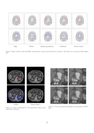
19. Global Narrow band 1
Figure 19: Deformable mesh (top) and 3D level set surface (bottom)
in 3D abdominal CT
Global Narrow band 1 the vicinity of the target object. Based on the theory of
parallel curves and surfaces, a mathematical development
Figure 18: Slices of deformable mesh (top) and 3D level set surface was carried out in order to express the region energies in a
(bottom) on axial planes of a 3D abdominal CT form allowing natural implementation on explicit models.
The distinctive feature of the 2D region term resides in
curvature. By extension, the region term employed in the
We eventually describe experiments made with the 3D mesh uses mean and gaussian curvatures. The narrow
active surface model on 3D CT datasets of the abdomen. band region energy managed to overcome the drawbacks
The surface is used to segment the inside of the whole of deformable models relying exclusively on edge terms or
aorta, in the context of abdominal aortic aneurysm global region terms. We provided explicit and level-set
diagnosis. It is initialized as a sphere totally inside based implementations in 2D and 3D. Very promising
the vessel and inflated afterwards. These experiments results were obtained on grayscale and color images.
emphasize the ability of our explicit active surface to
explore tree-like structures with narrow paths while Several improvements will be considered in the near fu-
keeping sufficient regularity. Endowed with the global ture. First, the bias added to the region force, described in
region-term, we observe the same phenomenon as with section 5.5, comes more from empirical observations rather
the active contour in 2D CT images. The surface tends than rigorous calculus of energy variations. Narrow band
to flow into neighboring structures which have a signifi- region-based models have a diminished capture range and
cantly brighter intensity than the background, especially the bias prevents the model to be stuck in a local mini-
when areas are separated by thin boundaries. On this mum when inner and outer statistics are similar. Future
data, such case appears between the white blood aorta work may concentrate on exploiting both global and band-
and vertebrae. Fig. 18 shows an axial slice of a 3D based region features, in order to dispense the use of such
abdominal CT dataset whereas the 3D representation bias. Moreover, further investigations will be performed
appears in fig. 19. The image size is 512 × 512 × 800, in embedding narrow region terms into more geometrically
yielding a computational time of nearly 55s for the de- constrained models, like the deformable generalized cylin-
formable mesh and more than 3mn for the implicit surface. der in [51]. We also plan to extend the model to temporal
segmentation, in order to track evolving objects in videos,
and to textured images [25]. Finally, automated learning
of the energy weights and band thickness, with respect to
8. Conclusion a given class of images, could be considered.
We have presented in this paper a narrow band region
approach for deformable contours and surfaces driven by A. Transformation of area and volume integrals
energy minimization. The approach is based on two novel In this appendix, we provide details about the trans-
region terms, formulating a homogeneity criterion in inner formations of area and volume integrals over 2D and 3D
and outer bands neighboring the evolving curve or surface. bands, respectively. These transformations lead to mathe-
The first and second term relies on the asumption of a matical expressions which discretized forms are convenient
respectively uniform and piecewise uniform background in to implement on explicit active contours and surfaces.
19

20. A.1. Area integral over 2D band We apply the same derivation on the term depending on Q,
We give a general form for an area integral over a which results in:
band B bounded by two non-intersecting simple curves Γ1 1
and Γ2 , as depicted in fig. 4. The curves enclose re- J(f, B) = ∇P (˜), xu cα − xα cu dαdu
c ˜ ˜ ˜ ˜
Ω 0
gions R1 and R2 , respectively. According to Green’s theo- 1
rem, since B = R1 R2 , the integral of a R2 → R function f + ∇Q(˜), yu cα − yα cu dαdu
c ˜ ˜ ˜ ˜
Ω 0
over B is:
Using simplifications
J(f, B) = J(f, R1 ) − J(f, R2 )
∂P 1 ∂Q 1
= x1 u P (c1 ) + y1 u Q(c1 )du =− f = f,
∂y 2 ∂x 2
Ω
− x2 u P (c2 ) + y2 u Q(c2 )du and rewriting with cross product, the final expression of
Ω the area integral is
where P and Q are the anti-derivatives defined in eq. (13). 1
We gather the terms depending on P and Q: J(f, B) = f (˜)(c1 − c2 ) × cu dαdu
c ˜ (58)
Ω 0
J(f, B) = x1u P (c1 ) − x2u P (c2 )du A.2. Area integral over inner band
Ω We apply the general result in eq. (58) on inner
+ y1 u Q(c1 ) − y2 u Q(c2 )du band Bin , considering curves Γ and Γ[B] instead of Γ1
Ω and Γ2 . Equations 7 and 11 give the substitutions:
˜
We introduce a family of curves {Γ(α)}α∈[0,1] interpolating c1 = c
˜
from Γ1 to Γ2 . The position vector of a given curve Γ(α) c2 = c + Bn
is c1u = cu
c(α, u) = (1 − α)c2 (u) + αc1 (u)
˜ c2u = (1 − Bκ)cu
This property allows us to write: Using the identity cu × n = −n × cu = ℓ, we obtain:
α=1 (c1 − c2 ) × ((1 − α)c2u + αc1u )
x1 u P (c1 ) − x2 u P (c2 ) = xu P (˜)
˜ c = (c − (c + Bn)) × ((1 − α)(1 − Bκ)cu + αc)
α=0
= Bℓ(Bκ(α − 1) − 1)
1
d
= xu P (˜) dα
˜ c Combined with eq. (16), this result yields:
0 dα
1
and similarly for y1 u Q(c1 ) − y2 u Q(c2 ). We have: J(f, Bin ) = f (c + B(α − 1)n)Bℓ(Bκ(α − 1) − 1)dαdu
Ω 0
1
d
J(f, B) = xu P (˜) + yu Q(˜) dαdu
˜ c ˜ c Introducing a variable thickness b = B(1 − α), ( dα = −
Ω 0 dα db / B ), we finally get:
1
B
= xαu P (˜) + yαu )Q(˜)dαdu
˜ c ˜ c
Ω 0 J(f, Bin ) = f (c + bn)ℓ(1 − bκ)dbdu
1 Ω 0
+ xu cα , ∇P (˜) + yu cα , ∇Q(˜) dαdu
˜ ˜ c ˜ ˜ c
Ω 0 A.3. Volume integral over 3D band
with cα = c1 − c2 . Integrating by parts the term
˜ We give a general form for an area integral over a volu-
depending on P with respect to u, we obtain: mic band B bounded by two non-intersecting surfaces Γ1
and Γ2 , enclosing regions R1 and R2 , respectively. The
u=1 mathematical derivation presented here may be consid-
xαu P (˜)du
˜ c = xα P (˜)
˜ c ered as the 3D extension of appendix A.1. Region R2 is
Ω u=0
d fully contained into R1 , such that B = R1 R2 . According
− xα
˜ P (˜) du
c to the divergence theorem described in eqs. (30) and (32),
Ω du
the integral of a R3 → R function f over B is:
Since Γ1 and Γ2 are closed curves, resulting in c1 (0) = J(f, B) = J(f, R1 ) − J(f, R2 )
c1 (1) and c1u (0) = c1u (1) and similarly for c2 , the bound-
ary term vanish: = F(s2 (u, v)), s2u ×s2v dudv
Ω2
xαu P (˜)du = −
˜ c xα cu , ∇P (˜) du
˜ ˜ c − F(s1 (u, v)), s1u ×s1v dudv
Ω Ω
Ω2
20

21. where F is the vector field [P Q R]T defined in eq. (33). Since the scalar triple product is anti-symetrical, we have
Introducing a variable surface of position vector ˜(α) in-
s
1
terpolating from Γ1 to Γ2 as α varies from 0 to 1, such J2 = ˜αu , ˜v × F + ˜αv , F × ˜u dαdudv
s s s s
that 0
Ω2
˜(α, u, v) = (1 − α)s1 (u, v) + αs2 (u, v),
s
we have: We integrate by parts the first and second terms with re-
spect to u and v, respectively:
F(s2 ), s2u ×s2v − F(s1 ), s1u ×s1v
1 1 u=1
α=1 1
d J2 = ˜α , ˜v ×F
s s dαdv
= F(˜)˜u טv
ss s = F(˜)˜u טv dα
ss s
α=0 0 dα 0 0 u=0
1
d
This yields: − ˜α ,
s ˜v ×F
s dαdudv
0 du
Ω2
1 1 1 v=1
d
J(f, B) = F(˜), ˜u טv
s s s dαdudv + ˜α , Fטu
s s dαdu
0 dα 0 0 v=0
Ω2 1
d
− ˜α ,
s Fטu
s dαdudv
Using the product rule to expand the α-derivative, J(f, B) 0 dv
is split into two terms: Ω2
The boundary terms vanish thanks to the surface param-
J(f, B) = J1 + J2
eterization, according to eq. (20) or (21). Expanding the
Integral J1 depends on the partial derivatives of F: cross product derivatives, we get:
1
1
dF(˜)
s dF(˜)
s
J1 = , ˜u טv dαdudv
s s J2 = − ˜α , ˜uv ×F + ˜v ×
s s s dαdudv
dα 0 du
0 Ω2
Ω2 1
dF(˜)
s
− ˜α ,
s טu + Fטuv dαdudv
s s
where dF(˜)/dα is a vector, expressed using partial deriva-
s 0 dv
Ω2
tives of application F: 1
T
= − ˜α , ˜v ×(∇F˜u ) + (∇F˜v )טu dαdudv
s s s s s
dF(˜)
s d˜s d˜
s d˜
s 0
= , ∇P , ∇Q , ∇R Ω2
dα dα dα dα
= ∇F˜α
s In the previous equation, the second member of the inner
product is expanded as a function of ˜u טv :
s s
where ∇F is the following Jacobian matrix:
    ˜v ×(∇F˜u ) + (∇F˜v )טu
s s s s
∂P ∂P ∂P 1 ∂P ∂P 
∂Q ∂R ∂Q ∂R

f − −
 ∂x ∂y ∂z   3 ∂y ∂z   ∂y ∂z ∂x ∂x 
 ∂Q ∂Q ∂Q   ∂Q 1 ∂Q   
∇F = 
  
f
 ∂P ∂P ∂R ∂R
=  =

− −

 ˜u טv
s s
 ∂x ∂y ∂z   ∂x 3 ∂z   ∂y ∂x ∂z ∂y 
 ∂R ∂R ∂R   ∂R ∂R 1 
f
 ∂P ∂Q ∂P ∂Q 
∂x ∂y ∂z ∂x ∂y 3 − −
∂z ∂z ∂x ∂y
Using matrix notation, we use the general rule which is rewritten in a form containing the divergence of
vector field:
aT Ab = (aT Ab)T = bT Aa
˜v ×(∇F˜u ) + (∇F˜v )טu = ∇FT − div(F)I ˜u טv
s s s s s s
to rewrite the integrand of J1 with inner product notation:
where I is the 3 × 3 identity matrix. It yields, for inte-
∇F˜α , ˜u טv = ˜α , ∇FT ˜u טv
s s s s s s gral J2 :
On the other hand, integral J2 depends explicitly on F: 1
J2 = ˜α , div(F)I − ∇FT ˜u טv dαdudv
s s s
1
d 0
J2 = F, ˜u טv
s s dαdudv Ω2
0 dα
Ω2
1
= F, ˜αu טv + F, ˜u טαv dαdudv
s s s s
0
Ω2
21

22. As a result, J1 and J2 are now straightforward to add: which yields, for J(f, Bin ):
1
J(f, B) = J1 + J2
1 J(f, Bin ) =
= ˜α , ∇FT ˜u טv
s s s Ω2
0
0
Ω2
Bf (s+αBn) su ×sv (1 − 2αBκM + α2 B 2 κG ) dαdudv
+ div(F)I − ∇FT ˜u טv dαdudv
s s
1
Introducing a variable thickness b = αB, we get the final
= div(F) ˜α , ˜u טv dαdudv
s s s
0
form of J(f, Bin ):
Ω2
J(f, Bin ) =
Eventually we give the final expression of the volume in- B
tegral: f (s + bn) su ×sv (1 − 2bκM + b2 κG )dbdudv
0
1 Ω2
J(f, B) = f (˜) s2 − s1 , ˜u טv dαdudv
s s s (59)
0
Ω2 B. Calculus of variations
This expression is intuitively understood as the scalar In this section, we calculate the variational derivative
triple product is the volume of the infinitesimal paral- of the region term J(f, Rin[B] ) with respect to contour po-
lelepiped spanned by vectors s2 − s1 , ˜u and ˜v .
s s sition c.
A.4. Volume integral over 3D inner band B.1. Variational derivative: general expression
We apply the result in eq. (59) on surfaces Γ and Γ[B] We consider the general energy functional, depending
instead of Γ1 and Γ2 , in order to provide a general ex- on the parallel curve Γ[B]
pression for J(f, Bin ). Thanks to equations 24 and 28, we
apply the substitutions: E= L(c[B] , c[B] u )du
Ω
s1 = s
s2 = s + Bn As is, the variational derivative of E with respect to posi-
s1u ×s1v = su ×sv tion vector c is difficult to write, but it is straightforward
s2 u ×s2 v = (1 − 2BκM + B 2 κG )su ×sv to express it with respect to the parallel position vector
c[B] :
which yields, in eq. (59): δE ∂L d ∂L
= −
δΓ[B] ∂c[B] du ∂c[B] u
s2 − s1 , ˜u טv
s s
= s[B] − s, ((1 − α)su + αs[B] u )×((1 − α)sv + αs[B] v ) The purpose here is to express δE/δc as a function of
δE/δc[B] , for a general energy term L. To some extent,
= Bn , (1 − α)2 su ×sv we design a chain rule for the variational derivatives of
parallel curve-based energies. In what follows, a partial
+α(1 − α)(su ×s[B] v + s[B] u ×sv ) + α2 s[B] u ×s[B] v derivative containing vector quantities should be under-
stood as a matrix:
= Bn , (1 − α)2 su ×sv  ∂a ∂a  x y
+α(1 − α)(2su ×sv + B(su ×nv + nu ×sv )) ∂a  ∂bx ∂bx 
=  ∂a ∂ay 
+α2 s[B] u ×s[B] v ∂b x
∂by ∂by
Thanks to eq. (27) and (28), this reduces to: The partial derivative of a scalar quantity with respect to
a position vector (or a derivative of this position vector)
s2 − s1 , ˜u טv
s s is the column vector:
su ×sv
= B , (1 − α)2 su ×sv ∂L ∂L ∂L
T
su ×sv =
+α(1 − α)(2su ×sv − 2Bsu ×sv ) ∂c ∂x ∂y
+α2 (1 − 2BκM + B 2 κG )su ×sv We expand the partial derivatives of L with the chain rule.
= B su ×sv (1 − 2αBκM + α B κG ) 2 2 First, we differentiate with respect to c:
∂L ∂c[B] ∂L
= (60)
∂c ∂c ∂c[B]
22

23. and cu :
∂L ∂c[B] ∂L ∂c[B] u ∂L ∂c[B] u xu xu κ yu ℓu yu
= + = +B − 3 t− (1 − Bκ)n
∂cu ∂cu ∂c[B] ∂cu ∂c[B] u ∂xu ℓ ℓ ℓ ℓ
∂c[B] u yu yu κ xu ℓu xu
which yields = +B + 3 t+ (1 − Bκ)n
∂yu ℓ ℓ ℓ ℓ
d ∂L ∂c[B] ∂L ∂c[B] ∂L
= +
du ∂cu ∂cu u ∂c[B] ∂cu ∂c[B] u ∂c[B] u Byu ∂c[B] u Bxu
(61) = 2 t =− 2 t
∂c[B] u ∂L ∂c[B] u ∂L ∂xuu ℓ ∂yuu ℓ
+ +
∂cu u ∂c[B] u ∂cu ∂c[B] u
u
∂c[B] u xu κ yu ℓu Byu κ
With respect to cuu , we have: =B − 3 t+ n
∂xuu u ℓ ℓ ℓ
∂L ∂c[B] u ∂L ∂c[B] u
= yu κ xu ℓu Bxu κ
∂cuu ∂cuu ∂c[B] u =B + 3 t− n
∂yuu u ℓ ℓ ℓ
which gives:
Incidentally, the following relation is verified:
d2 ∂L ∂c[B] u ∂L
2 ∂c = ∂c[B] u ∂c[B] u
du uu ∂cuu uu ∂c[B] u =
∂cu u ∂cuu uu
∂c[B] u ∂L ∂c[B] u ∂L
+2 +
∂cuu u ∂c[B] u ∂cuu ∂c[B] u The previous forms allow us to expand the underbraced
u uu
(62) terms in eq. (63):
Gathering (60), (61) and (62), we obtain:
∂L Bℓu ∂L
(1) = − 2 ,t n
δE ∂L ∂c[B] ∂L ∂c[B] ∂L ∂c[B] ℓ ∂c[B]
= − −
δΓ ∂c[B] ∂cu u ∂c[B] ∂cu ∂c[B] u ∂L ∂L
−Bκ , t t + Bκ ,n n
∂c[B] ∂c[B]
(1) (2)
∂c[B] u ∂c[B] u ∂L B ∂L
+ − (2) = − ,t n
∂cuu uu ∂cu u ∂c[B] u ℓ ∂c[B] u
(3) = 0
(3)
∂c[B] u ∂c[B] u ∂L (63)
+ 2 − ∂L Bℓu ∂L
∂cuu u ∂cu ∂c[B] u (4) = (Bκ−1) ,t t + 2 ,t n
u ∂c[B] u ℓ ∂c[B] u
u u
(4) ∂L
∂c[B] u −(1+Bκ) ,n n
∂L ∂c[B] u
+ u
∂cuu ∂c[B] u B ∂L
uu
(5) = − ,t n
(5) ℓ ∂c[B] u
uu
All derivatives of c[B] and c[B] u appearing in eq. (63) are We factorize:
expanded in the Frenet basis, where any vector x may be
expressed as a combination of tangent and normal vectors: δE ∂L ∂L
= (1−Bκ) − ,t t
δΓ ∂c[B] ∂c[B] u
x = x, t t + x, n n u
∂L ∂L
We have: + (1+Bκ) − ,n n
∂c[B] ∂c[B] u
∂c[B] ∂c[B] u
= [1 0]T = [0 1]T Bℓu ∂L ∂L
∂x ∂y − − ,t n
ℓ2 ∂c[B] ∂c[B] u
u
∂c[B] Byu ∂c[B] Bxu B ∂L ∂L
= 2 t =− 2 t + − ,t n
∂xu ℓ ∂yu ℓ ℓ ∂c[B] u ∂c[B] u
uu
∂c[B] xu κ yu ℓu Byu κ which is rewritten using the variational derivative of E
=B − 3 t+ n
∂xu u ℓ ℓ ℓ with respect to c[B] . We have the general formula,
∂c[B] yu κ xu ℓu Bxu κ which relates the variational derivatives with respect to c
=B + 3 t− n
∂yu u ℓ ℓ ℓ
23

24. and c[B] : [5] D. Adalsteinsson, J. Sethian, A fast level set method for prop-
agating interfaces, Journal of Computational Physics 118 (2)
δE δE δE (1995) 269–277.
= (1−Bκ) , t t + (1+Bκ) ,n n [6] D. Mumford, J. Shah, Optimal approximation by piecewise
δΓ δΓ[B] δΓ[B] smooth functions and associated variational problems, Com-
munications on Pure and Applied Mathematics 42 (5) (1989)
Bℓu δE B δE
− ,t n + ,t n 577–685.
ℓ2 δΓ[B] ℓ δΓ[B] u [7] T. Brox, D. Cremers, On the statistical interpretation of the
(64) piecewise smooth Mumford-Shah functional, in: International
Conference on Scale Space and Variational Methods in Com-
puter Vision (SSVM), Ischia, Italy, 2007, pp. 203–213.
B.2. Variational derivative: region integral over Rin [B] [8] R. Ronfard, Region based strategies for active contour models,
International Journal of Computer Vision 13 (2) (1994) 229–
The considered energy is now the area integral of any
251.
function f over the region enclosed by curve Γ[B] , ex- [9] J. Ivins, J. Porrill, Active region models for segmenting textures
pressed as a line integral using Green’s theorem: and colours, Image and Vision Computing 13 (5) (1995) 431–
438.
[10] S. Zhu, A. Yuille, Region competition: unifying snakes, re-
E = J(f, Rin[B] ) = x[B] u P (c[B] ) + y[B] u Q(c[B] )du gion growing, Bayes/MDL for multiband image segmentation,
Ω IEEE Transactions on Pattern Analysis and Machine Intelli-
gence 18 (9) (1996) 884–900.
Its variational derivative with respect to c[B] is easily de- [11] T. Chan, L. Vese, Active contours without edges, IEEE Trans-
termined from eq. (40), considering c[B] instead of c. One actions on Image Processing 10 (2) (2001) 266–277.
may find the complete mathematical derivation in the ap- [12] S. Jehan-Besson, M. Barlaud, G. Aubert, DREAM2 S: De-
pendix of [10]. formable regions driven by an eulerian accurate minimization
method for image and video segmentation, International Jour-
nal of Computer Vision 53 (1) (2003) 45–70.
δE y[B] u [13] N. Paragios, R. Deriche, Geodesic active regions and level set
= f (c[B] ) = −ℓ(1 − Bκ)f (c[B] )n (65)
δΓ[B] −x[B] u methods for motion estimation and tracking, Computer Vision
and Image Understanding 97 (3) (2005) 259–282.
Expression 64 needs the derivative of (65). Using the re- [14] G. Slabaugh, G. Unal, Active polyhedron: surface evolution
theory applied to deformable meshes, in: IEEE Computer Vi-
lation nu = − ℓκt, we get: sion and Pattern Recognition (CVPR), Vol. 2, San Diego, USA,
2005, pp. 84–91.
δE d [15] A. Dufour, V. Shinin, S. Tajbakhsh, N. Guill´n-Aghion, J.-C.
e
=− ℓ(1−Bκ)f (c[B] ) n Olivo-Marin, C. Zimmer, Segmenting and tracking fluorescent
δΓ[B] u du (66)
cells in dynamic 3-D microscopy with coupled active surfaces,
+ ℓ2 κ(1−Bκ)f (c[B] )t IEEE Transactions on Image Processing 14 (9) (2005) 1396–
1410.
We substitute eqs. (65) and (66) into 64. Since n, t = 0, [16] M. Taron, N. Paragios, M.-P. Jolly, Registration with uncer-
this reduces to: tainties and statistical modeling of shapes with variable metric
kernels, IEEE Transactions on Pattern Analysis and Machine
δE Intelligence 31 (1) (2009) 99–113.
= (1+Bκ) −ℓ(1−Bκ)f (c[B] ), n n [17] N. Paragios, R. Deriche, Geodesic active regions and level
δΓ
set methods for supervised texture segmentation, International
B d Journal of Computer Vision 46 (3) (2002) 223–247.
+ − ℓ(1−Bκ)f (c[B] ) n
ℓ du [18] J. Piovano, T. Papadopoulo, Local statistic based region seg-
mentation with automatic scale selection, in: European Confer-
+ℓ2 κ(1−Bκ)f (c[B] )t , t n ence on Computer Vision (ECCV), Vol. 5303 of LNCS, Springer,
Marseille, France, 2008, pp. 486–499.
[19] M. Alem´n-Flores, L. Alvarez, V. Caselles, Texture-oriented
a
which eventually leads to: anisotropic filtering and geodesic active contours in breast tu-
mor ultrasound segmentation, Journal of Mathematical Imaging
δE and Vision 28 (1) (2007) 81–97.
= −ℓ(1−Bκ)f (c[B] )n (67)
δΓ [20] C. Li, C. Kao, J. Gore, Z. Ding, Implicit active contours driven
by local binary fitting energy, in: IEEE Computer Vision and
Pattern Recognition (CVPR), Minneapolis, Minnesota, USA,
References 2007, pp. 17–22.
[21] S. Lankton, A. Tannenbaum, Localizing region-based active
[1] M. Kass, A. Witkin, D. Terzopoulos, Snakes: active contour contours, IEEE Transactions on Image Processing 17 (11)
models, International Journal of Computer Vision 1 (4) (1988) (2008) 2029–2039.
321–331. [22] M. Jacob, T. Blu, M. Unser, Efficient energies and algorithms
[2] Z. Zhang, F. Braun, Fully 3D active surface models with self- for parametric snakes, IEEE Transactions on Image Processing
inflation and self-deflation forces, in: IEEE Computer Vision 13 (9) (2004) 1231–1244.
and Pattern Recognition (CVPR), San Juan, Puerto Rico, 1997, [23] R. Kimmel, Fast edge integration, S. Osher and N. Paragios
pp. 85–90. (Eds), Springer-Verlag, 2003, Ch. invited chapter in Geometric
[3] J. Lachaud, A. Montanvert, Deformable meshes with automated Level Set Methods in Imaging, Vision and Graphics.
topology changes for coarse-to-fine three-dimensional surface [24] R. Goldenberg, R. Kimmel, M. Rivlin, E. an Rudzsky, Fast
extraction, Medical Image Analysis 3 (2) (1999) 187–207. geodesic active contours, IEEE Transactions on Image Process-
[4] R. Malladi, J. Sethian, B. Vemuri, Shape modeling with front ing 10 (10) (2001) 1467–1475.
propagation: a level set approach, IEEE Transactions on Pat- [25] C. Sagiv, N. Sochen, Y. Zeevi, Integrated active contours for
tern Analysis and Machine Intelligence 17 (2) (1995) 158–175.
24

25. texture segmentation, IEEE Transactions on Image Processing measurement of the cortex from 3D MR images using coupled
15 (6) (2006) 1633–1646. surfaces propagation, IEEE Transactions on Medical Imaging
[26] J. Mille, R. Bon´, P. Makris, H. Cardot, 2D and 3D deformable
e 18 (10) (1999) 927–937.
models with narrow band region energy, in: IEEE International [48] J. Ivins, J. Porrill, Constrained active region models for fast
Conference on Image Processing (ICIP), San Antonio, USA, tracking in color image sequences, Computer Vision and Image
2007, pp. 57–60. Understanding 72 (1) (1998) 54–71.
[27] R. Farouki, C. Neff, Analytic properties of plane offset curves, [49] A. Mansouri, A. Mitiche, C. Vazquez, Multiregion competition:
Computer Aided Geometric Design 7 (1-4) (1990) 83–99. a level set extension of region competition to multiple region
[28] A. Gray, Modern differential geometry of curves and surfaces image partitioning, Computer Vision and Image Understanding
with Mathematica, CRC Press, 2nd edition, 1997. 101 (3) (2006) 137–150.
[29] V. Caselles, R. Kimmel, G. Sapiro, Geodesic active contours, [50] L. Pi, C. Shen, F. Li, J. Fan, A variational formulation for
International Journal of Computer Vision 22 (1) (1997) 61–79. segmenting desired objects in color images, Image and Vision
[30] S. Kichenassamy, A. Kumar, A. Olver, P.and Tannenbaum, Computing 25 (9) (2007) 1414–1421.
A. Yezzi, Gradient flows and geometric active contour mod- [51] J. Mille, R. Bon´, L. Cohen, Region-based 2D deformable gen-
e
els, in: IEEE International Conference on Computer Vision eralized cylinder for narrow structures segmentation, in: Eu-
(ICCV), Boston, MA, USA, 1995, pp. 810–815. ropean Conference on Computer Vision (ECCV), Vol. 5303 of
[31] B. Appleton, H. Talbot, Globally optimal geodesic active con- LNCS, Springer, Marseille, France, 2008, pp. 392–404.
tours, Journal of Mathematical Imaging and Vision 23 (1)
(2005) 67–86.
[32] G. Elber, L. In-Kwon, K. Myung-Soo, Comparing offset curve
approximation methods, IEEE Computer Graphics and Appli-
cations 17 (3) (1997) 62–71.
[33] A. Pressley, Elementary differential geometry, Springer, 2002.
[34] M. do Carmo, Differential geometry of curves and surfaces,
Prentice-Hall, 1976.
[35] L. Cohen, I. Cohen, Finite element methods for active contour
models and balloons for 2D and 3D images, IEEE Transactions
on Pattern Analysis and Machine Intelligence 15 (11) (1993)
1131–1147.
[36] R. Goldenberg, R. Kimmel, M. Rivlin, E. an Rudzsky, Cor-
tex segmentation: a fast variational geometric approach, IEEE
Transactions on Medical Imaging 21 (2) (2002) 1544–1551.
[37] T. McInerney, D. Terzopoulos, A dynamic finite element sur-
face model for segmentation and tracking in multidimensional
medical images with application to cardiac 4D image analysis,
Computerized Medical Imaging and Graphics 19 (1) (1995) 69–
83.
[38] M. Desbrun, M. Meyer, P. Schr¨der, A. Barr, Implicit fairing
o
of irregular meshes using diffusion and curvature flow, in: 26th
ACM Conference on Computer Graphics and Interactive Tech-
niques (SIGGRAPH), Los Angeles, USA, 1999, pp. 317–324.
[39] M. Meyer, M. Desbrun, P. Schr¨der, A. Barr, Discrete differ-
o
ential geometry operators for triangulated 2-manifolds, in: In-
ternational Workshop on Visualization and Mathematics (Vis-
Math), Berlin-Dahlem , Germany, 2002, pp. 35–57.
[40] G. Charpiat, P. Maurel, J.-P. Pons, R. Keriven, O. Faugeras,
Generalized gradients: priors on minimization flows, Interna-
tional Journal of Computer Vision 73 (3) (2007) 325–344.
[41] J. Oliensis, Local reproducible smoothing without shrinkage,
IEEE Transactions on Pattern Analysis and Machine Intelli-
gence 15 (3) (1993) 307–312.
[42] G. Taubin, Curve and surface smoothing without shrinkage, in:
IEEE International Conference on Computer Vision (ICCV),
Boston, MA, USA, 1995, pp. 852–957.
[43] L. Staib, A. Chakraborty, J. Duncan, An integrated approach
for locating neuroanatomical structure from MRI, International
Journal of Pattern Recognition and Artificial Intelligence 11 (8)
(1997) 1247–1269.
[44] Y. Shi, W. Karl, Real-time tracking using level sets, in: IEEE
Computer Vision and Pattern Recognition (CVPR), Vol. 2, San
Diego, USA, 2005, pp. 34–41.
[45] G. Chung, L. Vese, Energy minimization based segmentation
and denoising using a multilayer level set approach, in: 5th
International Workshop on Energy Minimization Methods in
Computer Vision and Pattern Recognition (EMMCVPR), Vol.
3757 of LNCS, Springer, St. Augustine, FL, USA, 2005, pp.
439–455.
[46] C. Le Guyader, L. Vese, Self-repelling snakes for topology-
preserving segmentation models, IEEE Transactions on Image
Processing 17 (5) (2008) 767–779.
[47] X. Zeng, L. Staib, R. Schultz, J. Duncan, Segmentation and
25