Downloaded 18 times

![• The structures of tumor tissue in CT reflects their nature
• E.g., active cancer cells, angiogenesis, necrosis [Aerts2014]
• Underlying cancer-related genomics [Gevaert2012]
• Cancer ecosystem is composed of micro-habitats [Gatenby2013]
• Relates to cancer subtype, patient survival, response to treatment
PREDICTING CANCER TREATMENT SUCCESS](https://image.slidesharecdn.com/btaradiomics29-160819072138/75/A-3-D-Riesz-Covariance-Texture-Model-for-the-Prediction-of-Nodule-Recurrence-in-Lung-CT-4-2048.jpg)
![• Goal: image-based personalized phenotyping
• Use 3-D texture analysis to predict response to stereotactic ablative
radiotherapy (SABR)
• Surrogate slow, costly and invasive molecular analysis
• Related work [Ganeshan2013, Ravanelli2013, Mattonen2014, Depeursinge2015]
• 2-D and suboptimal texture operators (isotropic, single scale)
• No separate analysis of nodule components
PERSONALIZED PHENOTYPING
treatment failure
treatment success
quant. feat. #1
quant.feat.#2](https://image.slidesharecdn.com/btaradiomics29-160819072138/75/A-3-D-Riesz-Covariance-Texture-Model-for-the-Prediction-of-Nodule-Recurrence-in-Lung-CT-5-2048.jpg)
![TEXTURE OPERATORS
7
• Texture operators [Depeursinge2014]
• A -dimensional texture analysis approach is characterized by a set of
local operators centered at the position
• Each operator is local in the sense its response to an image only
depends on a subregion of
• The subregion is the support of the operator
N
d
L1 ⇥ · · · ⇥ Ld
L1
L2
M1
M2
·
m
m
L1 ⇥ · · · ⇥ Ld
I(k)
k 2 M1 ⇥ · · · ⇥ Md
M1
M2
L1
L2
gn
I(k)
gn(k, m)](https://image.slidesharecdn.com/btaradiomics29-160819072138/75/A-3-D-Riesz-Covariance-Texture-Model-for-the-Prediction-of-Nodule-Recurrence-in-Lung-CT-7-2048.jpg)
![TEXTURE OPERATORS
8
• Texture operators [Depeursinge2014]
• A -dimensional texture analysis approach is characterized by a set of
local operators centered at the position
• Each operator is local in the sense its response to an image only
depends on a subregion of
• The subregion is the support of the operator
• For each position , the operator is applied (e.g., multiplied) to the image,
yielding response maps:
N
d
L1 ⇥ · · · ⇥ Ld
L1
L2
M1
M2
·
m
m
m
L1 ⇥ · · · ⇥ Ld
I(k)
k 2 M1 ⇥ · · · ⇥ Md
M1
M2
L1
L2
)gn
I(k)
response map
gn(k, m)](https://image.slidesharecdn.com/btaradiomics29-160819072138/75/A-3-D-Riesz-Covariance-Texture-Model-for-the-Prediction-of-Nodule-Recurrence-in-Lung-CT-8-2048.jpg)
![TEXTURE OPERATORS
9
• Texture operators
• Example: response maps of
multi-scale operators
• Multi-directional operators:
scale 1 scale 2 scale 3 scale 4
g1 g2 g3 g4
IA IB
XX 2013 2
otation–
ar pixels
ovariant
elatively
N = 1 G ⇤ R(0,1) G ⇤ R(1,0)
N = 2 G ⇤ R(0,2) G ⇤ R(1,1) G ⇤ R(2,0)
TIONS ON IMAGE PROCESSING, VOL. XX, NO. XX, XX 2013 2
e operators’ outputs over the instances. Rotation–
BPs are obtained by using “uniform” circular pixels
hat are rotation–invariant [39]. Rotation–covariant
RIFT [31]) measures HOG orientations relatively
N = 1 G ⇤ R(0,1) G ⇤ R(1,0)
N = 2 G ⇤ R(0,2) G ⇤ R(1,1) G ⇤ R(2,0)](https://image.slidesharecdn.com/btaradiomics29-160819072138/75/A-3-D-Riesz-Covariance-Texture-Model-for-the-Prediction-of-Nodule-Recurrence-in-Lung-CT-9-2048.jpg)
![TEXTURE OPERATOR
10
• Locally-oriented 3-D steerable Riesz wavelets
• Rotation-invariant characterization of the local organization of image
directions (LOID) is important for characterizing local tissue architectures
[Depeursinge2014]
ael Unser
b)
reattentive texture segregation [3].
easily separated from L-shaped
patterns (left) are found to be more
can be distinguished by counting](https://image.slidesharecdn.com/btaradiomics29-160819072138/75/A-3-D-Riesz-Covariance-Texture-Model-for-the-Prediction-of-Nodule-Recurrence-in-Lung-CT-10-2048.jpg)
![TEXTURE OPERATOR
• Locally-oriented 3-D steerable Riesz wavelets
• th-order Riesz transform in 3-D in Fourier [Unser2011]
yields for all combinations of
N
✓
N + 2
2
◆
n1 + n2 + n3 = N, n1,2,3 2 N
R(n1,n2,n3){f}(!) = ( j)N
r
N!
n1!n2!n3!
!n1
1 !n2
2 !n3
3
||!||n1+n2+n3
ˆf(!),](https://image.slidesharecdn.com/btaradiomics29-160819072138/75/A-3-D-Riesz-Covariance-Texture-Model-for-the-Prediction-of-Nodule-Recurrence-in-Lung-CT-11-2048.jpg)
![TEXTURE OPERATOR
• Locally-oriented 3-D steerable Riesz wavelets
• th-order Riesz transform in 3-D in Fourier [Unser2011]
yields for all combinations of
• Example
N
✓
N + 2
2
◆
n1 + n2 + n3 = N, n1,2,3 2 N
R(n1,n2,n3){f}(!) = ( j)N
r
N!
n1!n2!n3!
!n1
1 !n2
2 !n3
3
||!||n1+n2+n3
ˆf(!),
2
finition
of the
visual
ith the
expert
to find
ons of
k, and
s in a
G ⇤ R(2,0,0)
G ⇤ R(0,2,0)
G ⇤ R(0,0,2)
G ⇤ R(1,1,0)
G ⇤ R(1,0,1)
G ⇤ R(0,1,1)
N = 2
' ⇤ R(2,0,0)
' ⇤ R(0,2,0)
' ⇤ R(0,0,2)
' ⇤ R(0,1,1)
' ⇤ R(1,0,1)
' ⇤ R(1,1,0)](https://image.slidesharecdn.com/btaradiomics29-160819072138/75/A-3-D-Riesz-Covariance-Texture-Model-for-the-Prediction-of-Nodule-Recurrence-in-Lung-CT-12-2048.jpg)
![TEXTURE OPERATOR
13
• Locally-oriented 3-D steerable Riesz wavelets
• th-order Riesz transform in 3-D in Fourier [Unser2011]
yields for all combinations of
• Steerability [Chenouard2012]
is a rotation matrix and is the corresponding steering matrix
N
✓
N + 2
2
◆
n1 + n2 + n3 = N, n1,2,3 2 N
RN
{fR} = SRRN
{f}
R 3 ⇥ 3 SR
R(n1,n2,n3){f}(!) = ( j)N
r
N!
n1!n2!n3!
!n1
1 !n2
2 !n3
3
||!||n1+n2+n3
ˆf(!),](https://image.slidesharecdn.com/btaradiomics29-160819072138/75/A-3-D-Riesz-Covariance-Texture-Model-for-the-Prediction-of-Nodule-Recurrence-in-Lung-CT-13-2048.jpg)
![TEXTURE OPERATOR
14
• Locally-oriented 3-D steerable Riesz wavelets
• th-order Riesz transform in 3-D in Fourier [Unser2011]
yields for all combinations of
• Steerability [Chenouard2012]
is a rotation matrix and is the corresponding steering matrix
• Spatial support
• Isotropic dyadic wavelet frames
N
✓
N + 2
2
◆
n1 + n2 + n3 = N, n1,2,3 2 N
RN
{fR} = SRRN
{f}
R 3 ⇥ 3 SR
R(n1,n2,n3){f}(!) = ( j)N
r
N!
n1!n2!n3!
!n1
1 !n2
2 !n3
3
||!||n1+n2+n3
ˆf(!),
of order −1/2 (an isotropic smoothing operator) of f: Rf =
−∇∆−1/2
f. Let’s indeed recall the Fourier-domain definition of
these operators: ∇
F
←→ jω and ∆−1/2 F
←→ ||ω||−1
. Unlike the
usual gradient ∇, the Riesz transform is self-reversible
R⋆
Rf(ω) =
(jω)∗
(jω)
||ω||2
ˆf(ω) = ˆf(ω).
This allows us to define a self-invertible wavelet frame of L2(R3
)
(tight frame). We however see that there exists a singularity for the
frequency (0, 0, 0). This issue will be fixed later, thanks to the van-
ishing moments of the primary wavelet transform.
RN
{f ⇤ i}[k]
ˆi(!)
⇡
2i
L1 ⇥ L2 ⇥ L3](https://image.slidesharecdn.com/btaradiomics29-160819072138/75/A-3-D-Riesz-Covariance-Texture-Model-for-the-Prediction-of-Nodule-Recurrence-in-Lung-CT-14-2048.jpg)
![TEXTURE OPERATOR
15
• Locally-oriented 3-D steerable Riesz wavelets
• Rotation-invariant characterization of the local organization of image
directions (LOID) is important for characterizing local tissue architectures
[Depeursinge2014]
• The structure tensor is used to estimate the orientation that maximizes the
response of at each position [Chenouard2012]
• The sorted collection of eigenvectors of defines a rotation matrix
and a corresponding steering matrix
• Our texture operator is
• It characterizes the LOIDs in a rotation-invariant fashion [Dicente2016]
R
R[m]J[m]
m
J[m] =
0
@
R2
1{' ⇤ f}[m] R1R2{' ⇤ f}[m] R1R3{' ⇤ f}[m]
R1R2{' ⇤ f}[m] R2
2{' ⇤ f}[m] R2R3{' ⇤ f}[m]
R1R3{' ⇤ f}[m] R2R3{' ⇤ f}[m] R2
3{' ⇤ f}[m]
1
A
gn[f[k], m] = SR[m]RN
{f ⇤ i}
SR[m]
• Locally-oriented 3D Riesz wavelets [Chenouard2012,Depeursinge2015]
• Operator: directional filters behaving like local partial image derivatives
• E.g. second-order:
• Suitable for exploring first- and higher-order transitions between voxel values
• Multi-scale (wavelets)
• Steerable
• Finds the 3D direction maximizing local image derivatives
• Combines directional analysis with rotation-invariance
PROPOSED 3D TEXTURE FEATURES
l
an ensemble of examples called the training set.28
Once the SVM model
has been built from the example cases, it can predict the class of an un-
seen case with a confidence score (called computer score thereinafter).
The group of variables feeding SVMs consisted of the responses (ie,
energies) of the multiscale Riesz filters in each of the 36 anatomical re-
gions of the lungs (Fig. 3). The size of the vector vl regrouping the re-
sponses of the 6 Riesz filters at 4 scales from the 36 regions was
equal to 864.
To compare Riesz wavelets with other features that could capture
the radiological phenotype of diffuse lung disease, 2 different feature
groups were extracted for each region to provide a baseline performance:
15 histogram bins of the gray levels in the extended lung window
[−1000; 600] Hounsfield units (HU) and 3D gray-level co-occurrence
matrices (GLCM).29
Statistical measures from GLCMs are popular tex-
ture attributes that were used by several studies in the literature to
in {−3; 3} and {8, 16, 32}, respectively. The size
butes vl was 540 for the gray-level histogram attrib
inafter) and 396 for the GLCM attributes.
RESULTS
A leave-one-patient-out cross-validation ev
estimate the performance of the proposed appr
patient-out cross-validation consisted of using all
the SVM model and to measure the prediction pe
maining test patient. The prediction performanc
over all possible combinations of training and t
operating characteristic (ROC) curves of the sys
classifying between classic and atypical UIP are s
different feature groups and their combinations. T
obtained by varying the decision threshold betwe
FIGURE 2. Second-order Riesz filters characterizing edges along the main image directions X, Y, Z and 3 diagonals XY, XZ, and YZ. F
online in color at www.investigativeradiology.com.
© 2014 Wolters Kluwer Health, Inc. All rights reserved. www.investigative
Copyright © 2014 Wolters Kluwer Health, Inc. Unauthorized reproduction of this article is prohibited.
@2
@x2
@2
@y2
@2
@z2
@2
@x@y
@2
@x@z
@2
@y@z
scale 1 scale 2](https://image.slidesharecdn.com/btaradiomics29-160819072138/75/A-3-D-Riesz-Covariance-Texture-Model-for-the-Prediction-of-Nodule-Recurrence-in-Lung-CT-15-2048.jpg)
![FEATURE MAPS AND AGGREGATION FUNCTIONS
• From texture operators to texture measurements
• The operator is typically applied to all positions of the image
by “sliding” its window over the image
• Yields feature maps (potentially concatenating outputs from several operators)
• Regional texture measurements can be obtained from the aggregation of
over a region of interest
• E.g., provide estimates of features statistics
L1
L2
M1
M2
L1 ⇥ · · · ⇥ Ld
·
m
M
M
m
gn[k, m]
gn[f[k], m]
Mmargin
Mtexture](https://image.slidesharecdn.com/btaradiomics29-160819072138/75/A-3-D-Riesz-Covariance-Texture-Model-for-the-Prediction-of-Nodule-Recurrence-in-Lung-CT-17-2048.jpg)
![• For instance, integration can be used to aggregate the vectors
over
• Average
• The average of absolute values can be used for bandlimited operators
INTEGRATIVE AGGREGATION FUNCTIONS
18
M
• From texture operators to texture measurements
• The operator is typically applied to all positions
by “sliding” its window over the image
• Regional texture measurements can be obtained
aggregation of over a region of interest
• For instance, integration can be used to aggregate
• e.g., average:
L1
L2
M1
M2
L1 ⇥ · · · ⇥ Ld
·
gn(x, m)
µ 2 RP
gn(f(x), m) M
m
gn(f(x
µ =
0
B
@
µ1
...
µP
1
C
A =
1
|M|
Z
M
gn(f(x), m) p=1,...,P
dm
M
'm = gn[f[k], m] 2 RP
µ =
0
B
@
µ1
...
µP
1
C
A =
1
|M|
X
m2M
'm](https://image.slidesharecdn.com/btaradiomics29-160819072138/75/A-3-D-Riesz-Covariance-Texture-Model-for-the-Prediction-of-Nodule-Recurrence-in-Lung-CT-18-2048.jpg)
![INTEGRATIVE AGGREGATION FUNCTIONS
• How large must be the region of interest ?
• No more than enough to evaluate texture stationarity
in terms of human perception / tissue biology
• Example with operator: undecimated isotropic Simoncelli’s dyadic wavelets
[Portilla2000] applied to all image positions
• Operators’ responses are averaged over
M
• The operator is typically applied to all position
by “sliding” its window over the image
• Regional texture measurements can be obtained
aggregation of over a region of interest
• For instance, integration can be used to aggregate
• e.g., average:
L1
L2
M1
M2
L1 ⇥ · · · ⇥ Ld
·
gn(x, m)
µ 2 RP
gn(f(x), m) M
m
gn(f(
µ =
0
B
@
µ1
...
µP
1
C
A =
1
|M|
Z
M
gn(f(x), m) p=1,...,P
dm
M
f(x) g1(f(x), m)
m 2 RM1⇥M2
g2(f(x), m)
original image with
regions I
1
|M|
Z
M
|g1(f(x), m)|dm
M
feature space
1
|M|
Z
M
|g2(f(x),m)|dm
f(x)
Ma, Mb, Mc
The averaged responses
over the entire image
does not correspond
to anything visually!
ˆg1(⇢) =
⇢
cos ⇡
2 log2
2⇢
⇡ , ⇡
4 < ⇢ ⇡
0, otherwise.
ˆg2(⇢) =
⇢
cos ⇡
2 log2
4⇢
⇡ , ⇡
8 < ⇢ ⇡
2
0, otherwise.
g1,2 f(⇢, ) = ˆg1,2(⇢, ) · ˆf(⇢, )
Nor biologically!](https://image.slidesharecdn.com/btaradiomics29-160819072138/75/A-3-D-Riesz-Covariance-Texture-Model-for-the-Prediction-of-Nodule-Recurrence-in-Lung-CT-19-2048.jpg)
![• For instance, integration can be used to aggregate the vectors
over
• Average
• The average of absolute values can be used for bandlimited operators
• Covariance matrix
• Encodes pixelwise inter-feature variations [Cirujeda2015]
• Variance is a reasonable statistic for bandlimited operators
• Can be vectorized to keep unique elements as
INTEGRATIVE AGGREGATION FUNCTIONS
20
M
• From texture operators to texture measurements
• The operator is typically applied to all positions
by “sliding” its window over the image
• Regional texture measurements can be obtained
aggregation of over a region of interest
• For instance, integration can be used to aggregate
• e.g., average:
L1
L2
M1
M2
L1 ⇥ · · · ⇥ Ld
·
gn(x, m)
µ 2 RP
gn(f(x), m) M
m
gn(f(x
µ =
0
B
@
µ1
...
µP
1
C
A =
1
|M|
Z
M
gn(f(x), m) p=1,...,P
dm
M
'm = gn[f[k], m] 2 RP
= vec(X) = X1,1,
p
2X1,2, . . . ,
p
2X1,P , X2,2,
p
2X2,3, . . . XP,P
X =
1
|M| 1
X
m2M
('m µM )('m µM )T
µ =
0
B
@
µ1
...
µP
1
C
A =
1
|M|
X
m2M
'm
2 RP (P +1)/2](https://image.slidesharecdn.com/btaradiomics29-160819072138/75/A-3-D-Riesz-Covariance-Texture-Model-for-the-Prediction-of-Nodule-Recurrence-in-Lung-CT-20-2048.jpg)
![• Covariance matrices lie in Riemannian manifolds of real
symmetric positive definite matrices [Pennec2006]
• Euclidean distance between different texture regions fails
RIEMANNIAN MANIFOLDS
Sym+
P
Sym+
P
1
2
3
Mj
21](https://image.slidesharecdn.com/btaradiomics29-160819072138/75/A-3-D-Riesz-Covariance-Texture-Model-for-the-Prediction-of-Nodule-Recurrence-in-Lung-CT-21-2048.jpg)
![• Covariance matrices lie in Riemannian manifolds of real
symmetric positive definite matrices [Pennec2006]
• Euclidean distance between different texture regions fails
• Meaningful distances exist:
• e.g., [Förstner2003]:
where and are the elements of SVD of
Therefore:
where are the positive eigenvalues of
RIEMANNIAN MANIFOLDS
Sym+
P
Sym+
P
1
2
3
(X1, X2) =
s
trace
✓
log
⇣
X
1
2
1 X2X
1
2
1
⌘2
◆
,
log(X) = Ulog(D)UT
,
SVD of X: X=UDV^T
other distances:
Jensen-Bregman divergence
U D X 2 Sym+
P
(X1, X2) =
v
u
u
t
PX
i=1
log( i)2,
X
1
2
1 X2X
1
2
1i
Mj
22](https://image.slidesharecdn.com/btaradiomics29-160819072138/75/A-3-D-Riesz-Covariance-Texture-Model-for-the-Prediction-of-Nodule-Recurrence-in-Lung-CT-22-2048.jpg)
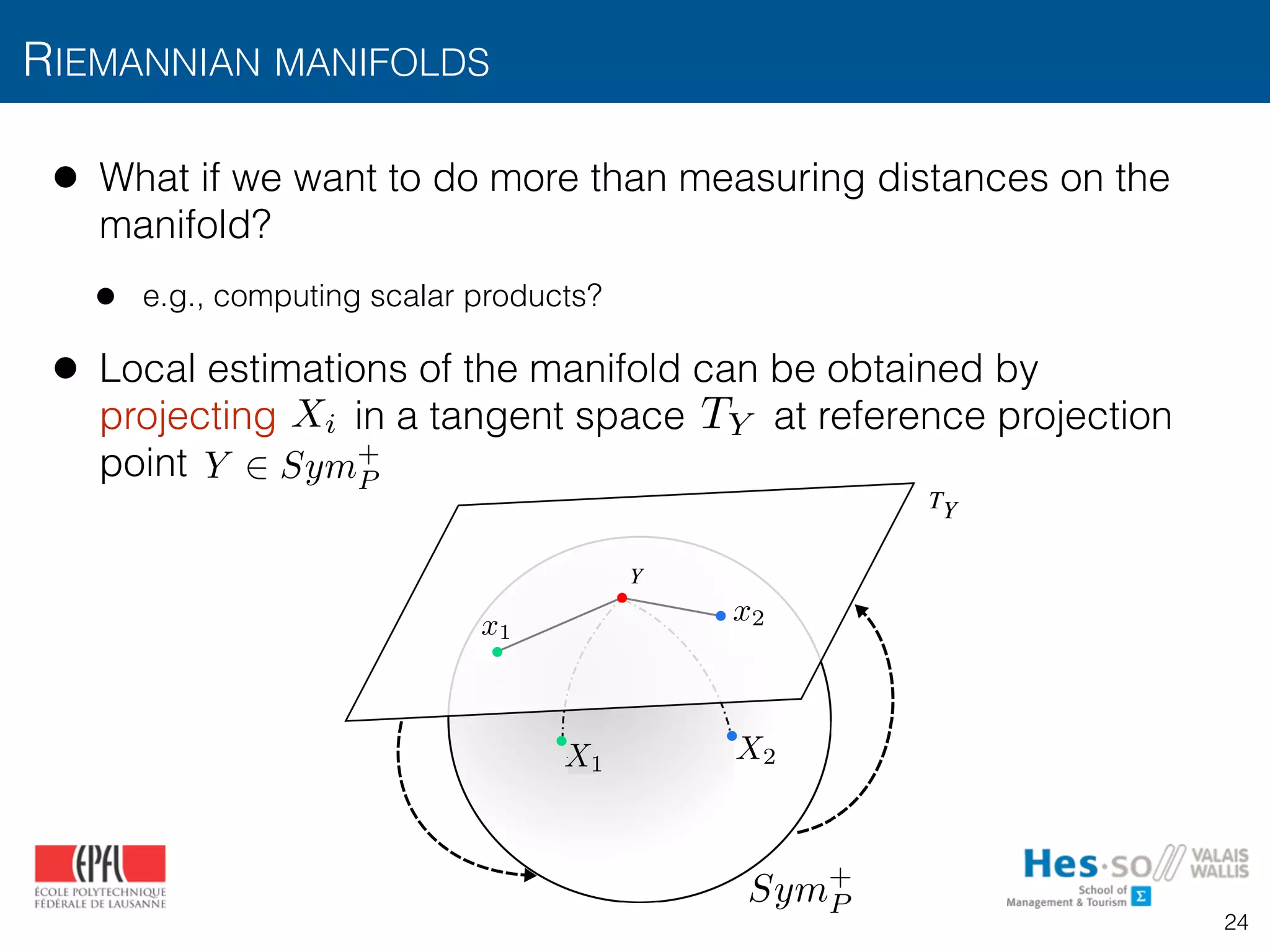
![• Projections are obtained by the point-dependent operation
[Arsigny2006]
and we can come back
RIEMANNIAN MANIFOLDS
logY
TY
expY
Fig. 3: Mapping of points in a Sym+
manifold to the tangent
Riemannian
tion demonst
covariance de
b) the provid
are able to
and c) this c
knowledge o
and recurrenc
X2X1
x2x1
Sym+
P
logY
expY
x = logY (X) = Y
1
2 log
⇣
Y
1
2 XY
1
2
⌘
Y
1
2
X = expY (x) = Y
1
2 exp
⇣
Y
1
2 xY
1
2
⌘
Y
1
2
25](https://image.slidesharecdn.com/btaradiomics29-160819072138/75/A-3-D-Riesz-Covariance-Texture-Model-for-the-Prediction-of-Nodule-Recurrence-in-Lung-CT-25-2048.jpg)
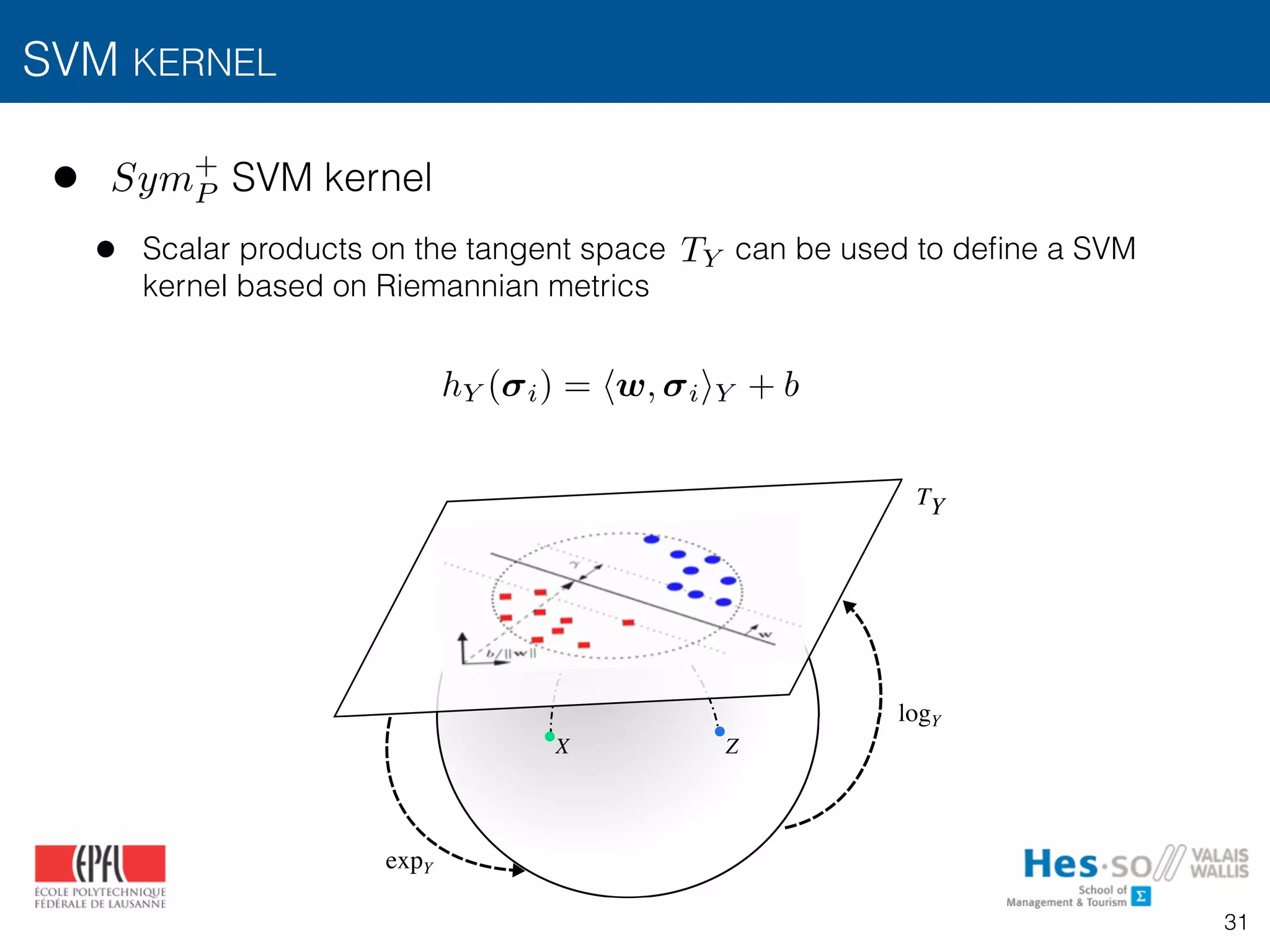
![• Now we can use the Euclidean metric on the tangent space
• Scalar product between two points and [Pennec2006]:
• It can be used to define a kernel for e.g., support vector machines (SVM)
RIEMANNIAN MANIFOLDS
logY
TY
expY
Fig. 3: Mapping of points in a Sym+
manifold to the tangent
Riemannian
tion demonst
covariance de
b) the provid
are able to
and c) this c
knowledge o
and recurrenc
X2X1
x2x1
Sym+
P
logY
expY
TY
x2x1
hx1, x2iY = trace x1Y 1
x2Y 1
26](https://image.slidesharecdn.com/btaradiomics29-160819072138/75/A-3-D-Riesz-Covariance-Texture-Model-for-the-Prediction-of-Nodule-Recurrence-in-Lung-CT-26-2048.jpg)
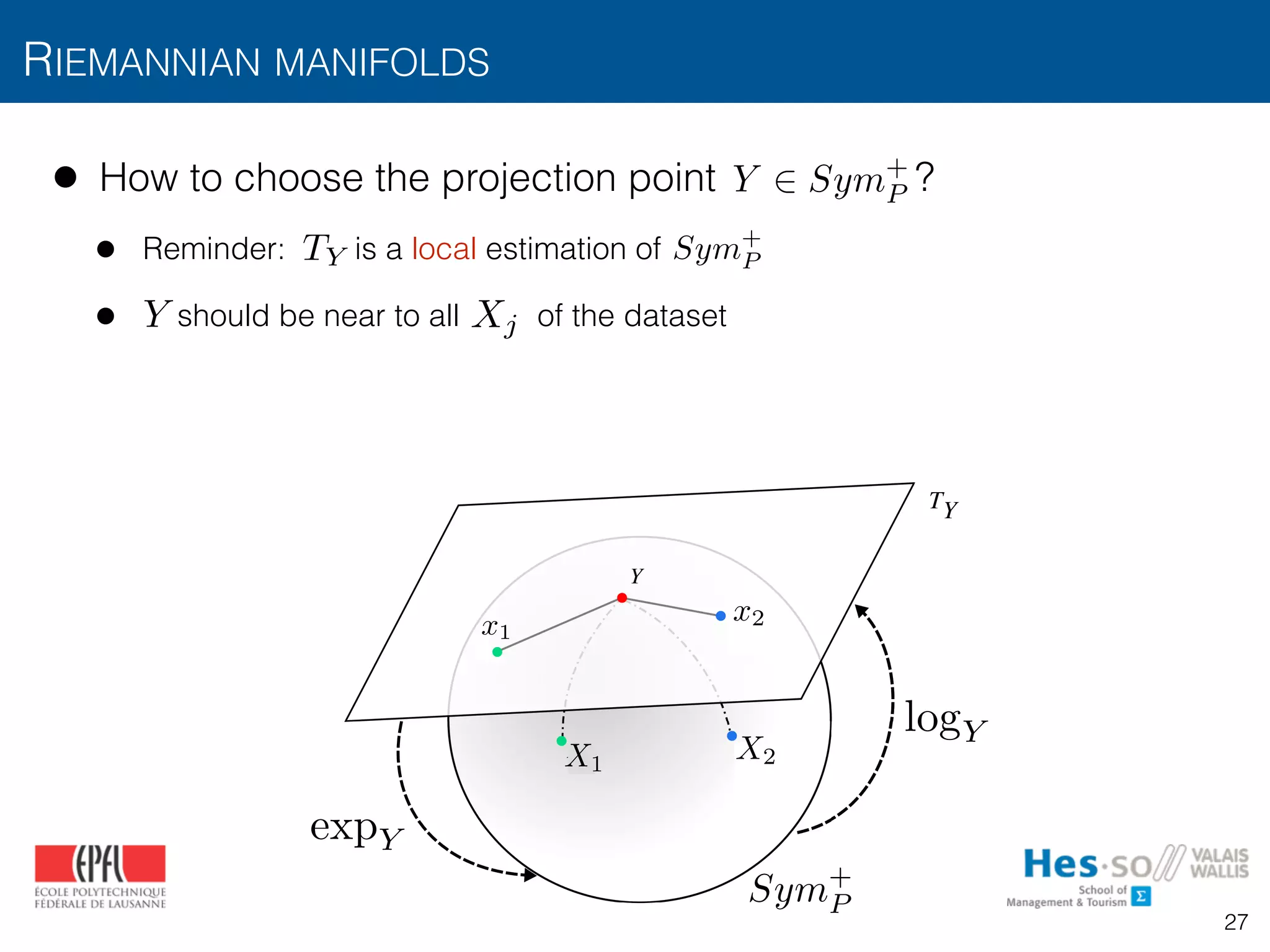
![• How to choose the projection point ?
• Reminder: is a local estimation of
• should be near to all of the dataset
• The mean of covariances is a natural choice [Pennec2006]:
• can be estimated with gradient descent and iterative re-projection
[Pennec2006, Karcher1977, Moakher2005]
• is convex
RIEMANNIAN MANIFOLDS
Y 2 Sym+
P
Sym+
PTY
Y Xj
Xµ : argmin
Xµ2Sym+
d
JX
j=1
2
(Xj, Xµ)
Y = Xµ
Xµ
Sym+
P
28](https://image.slidesharecdn.com/btaradiomics29-160819072138/75/A-3-D-Riesz-Covariance-Texture-Model-for-the-Prediction-of-Nodule-Recurrence-in-Lung-CT-28-2048.jpg)
![• Linear support vector machines (SVM) [Cortes1995]
• Finds the hyperplane with maximum margin using training instances
• Decision function for a test instance
SVM KERNEL
Machine `a vecteurs supports lin´eaire
R´eponse : La plus grande marge
b/∥w∥ γ
⟨w, x⟩ + b
γ
w
) Celui qui a la plus grande marge
b/||w||
w
w
30
i
h( i) = hw, ii + b](https://image.slidesharecdn.com/btaradiomics29-160819072138/75/A-3-D-Riesz-Covariance-Texture-Model-for-the-Prediction-of-Nodule-Recurrence-in-Lung-CT-30-2048.jpg)
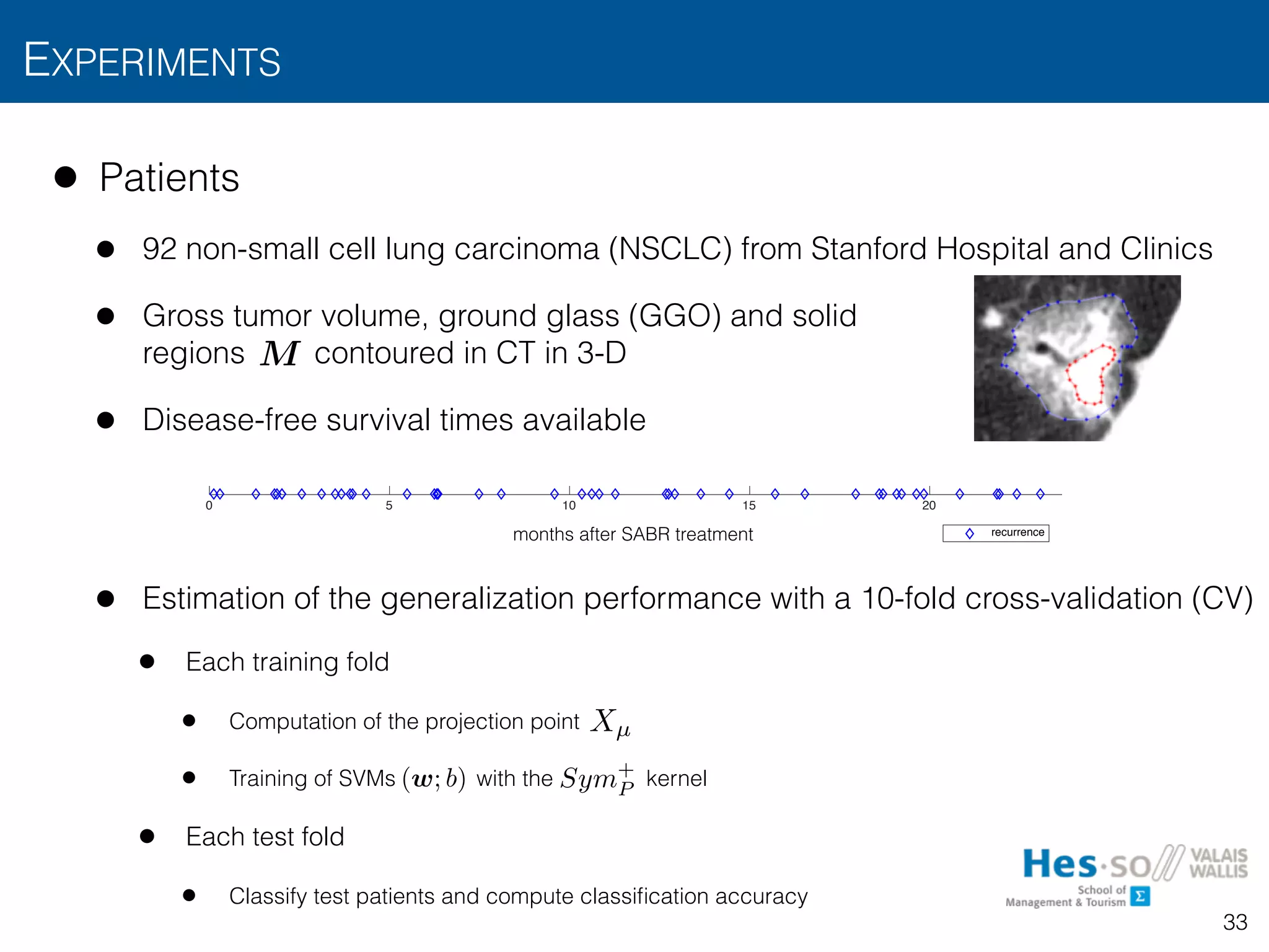
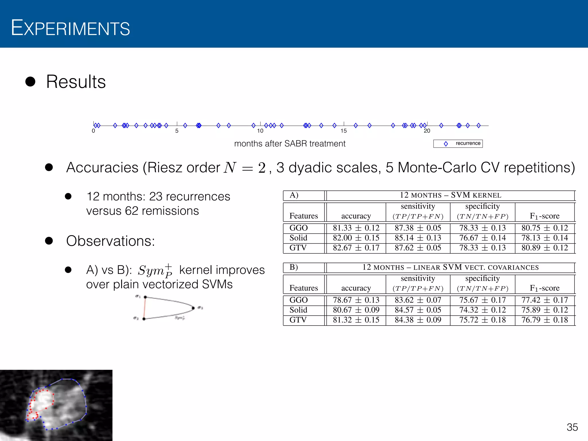
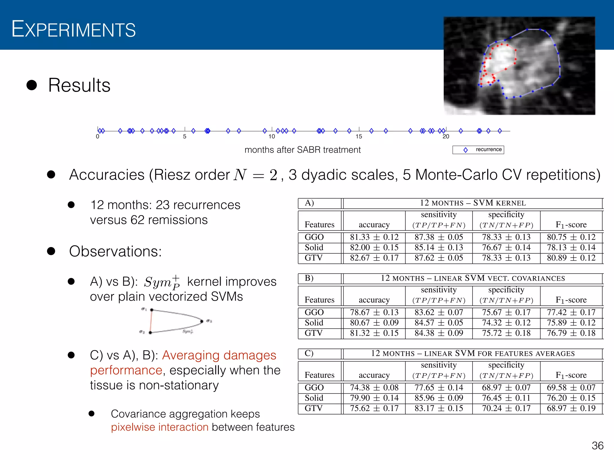
![• Results
• Accuracies (Riesz order , 3 dyadic scales, 5 Monte-Carlo CV repetitions)
• 12 months: 23 recurrences versus 62 remissions
• 24 months: 30 recurrences versus 62 remissions
• Observations
• Predicts treatment failure in first 12 months with accuracy > 80%
EXPERIMENTS
34
0 5 10 15 20
0
0.1
0.2
0.3
0.4
0.5
0.6
0.7
0.8
0.9
1
months after SABR treatment
0 5 10 15 20
0
0.1
0.2
0.3
0.4
0.5
0.6
0.7
0.8
0.9
1
recurrence
N = 2
9
TABLE I: Results for the binary classification of patient recurrence, using short– (12 months) and long–term (24 months)
binarization and several nodule region descriptors. Table A presents the performance evaluation of the presented kernel–based
SVM formulation for covariance-based descriptors. Table B shows the results of a linear SVM for plain vectorized covariance
descriptors. Finally, Table C assesses the performance of a linear SVM using the average of the 3–D Riesz filter responses
within the delineated region as templates (e.g., corresponding to our approach in [18]). The short–term experiment involved
23 recurrences versus 62 remissions. The long–term experiment involved 30 recurrences versus 62 remissions. Table values
are expressed in terms of CV repetition averages ± standard deviations.
A) 12 MONTHS – SVM KERNEL 24 MONTHS – SVM KERNEL
Features accuracy
sensitivity
(T P/T P +F N)
specificity
(T N/T N+F P ) F1-score accuracy
sensitivity
(T P/T P +F N)
specificity
(T N/T N+F P ) F1-score
GGO 81.33 ± 0.12 87.38 ± 0.05 78.33 ± 0.13 80.75 ± 0.12 54.94 ± 0.12 61.64 ± 0.14 58.51 ± 0.05 53.74 ± 0.07
Solid 82.00 ± 0.15 85.14 ± 0.13 76.67 ± 0.14 78.13 ± 0.14 57.33 ± 0.05 68.98 ± 0.08 50.89 ± 0.02 49.37 ± 0.03
GTV 82.67 ± 0.17 87.62 ± 0.05 78.33 ± 0.13 80.89 ± 0.12 44.69 ± 0.15 63.33 ± 0.22 47.80 ± 0.15 41.77 ± 0.10
B) 12 MONTHS – LINEAR SVM VECT. COVARIANCES 24 MONTHS – LINEAR SVM VECT. COVARIANCES
Features accuracy
sensitivity
(T P/T P +F N)
specificity
(T N/T N+F P ) F1-score accuracy
sensitivity
(T P/T P +F N)
specificity
(T N/T N+F P ) F1-score
GGO 78.67 ± 0.13 83.62 ± 0.07 75.67 ± 0.17 77.42 ± 0.17 49.63 ± 0.15 58.89 ± 0.05 56.92 ± 0.15 52.30 ± 0.16
Solid 80.67 ± 0.09 84.57 ± 0.05 74.32 ± 0.12 75.89 ± 0.12 57.33 ± 0.11 67.11 ± 0.06 58.01 ± 0.03 56.24 ± 0.09
GTV 81.32 ± 0.15 84.38 ± 0.09 75.72 ± 0.18 76.79 ± 0.18 44.87 ± 0.08 57.71 ± 0.11 48.76 ± 0.07 42.86 ± 0.09
C) 12 MONTHS – LINEAR SVM FOR FEATURES AVERAGES 24 MONTHS – LINEAR SVM FOR MEAN OF FEATURES TEMPLATE
Features accuracy
sensitivity
(T P/T P +F N)
specificity
(T N/T N+F P ) F1-score accuracy
sensitivity
(T P/T P +F N)
specificity
(T N/T N+F P ) F1-score
GGO 74.38 ± 0.08 77.65 ± 0.14 68.97 ± 0.07 69.58 ± 0.07 46.67 ± 0.25 50.00 ± 0.23 50.41 ± 0.23 46.41 ± 0.25
Solid 79.90 ± 0.14 85.96 ± 0.09 76.45 ± 0.11 76.20 ± 0.15 53.33 ± 0.20 55.90 ± 0.23 53.60 ± 0.18 52.04 ± 0.19
GTV 75.62 ± 0.17 83.17 ± 0.15 70.24 ± 0.17 68.97 ± 0.19 51.67 ± 0.15 53.62 ± 0.15 52.17 ± 0.16 46.80 ± 0.15](https://image.slidesharecdn.com/btaradiomics29-160819072138/75/A-3-D-Riesz-Covariance-Texture-Model-for-the-Prediction-of-Nodule-Recurrence-in-Lung-CT-34-2048.jpg)
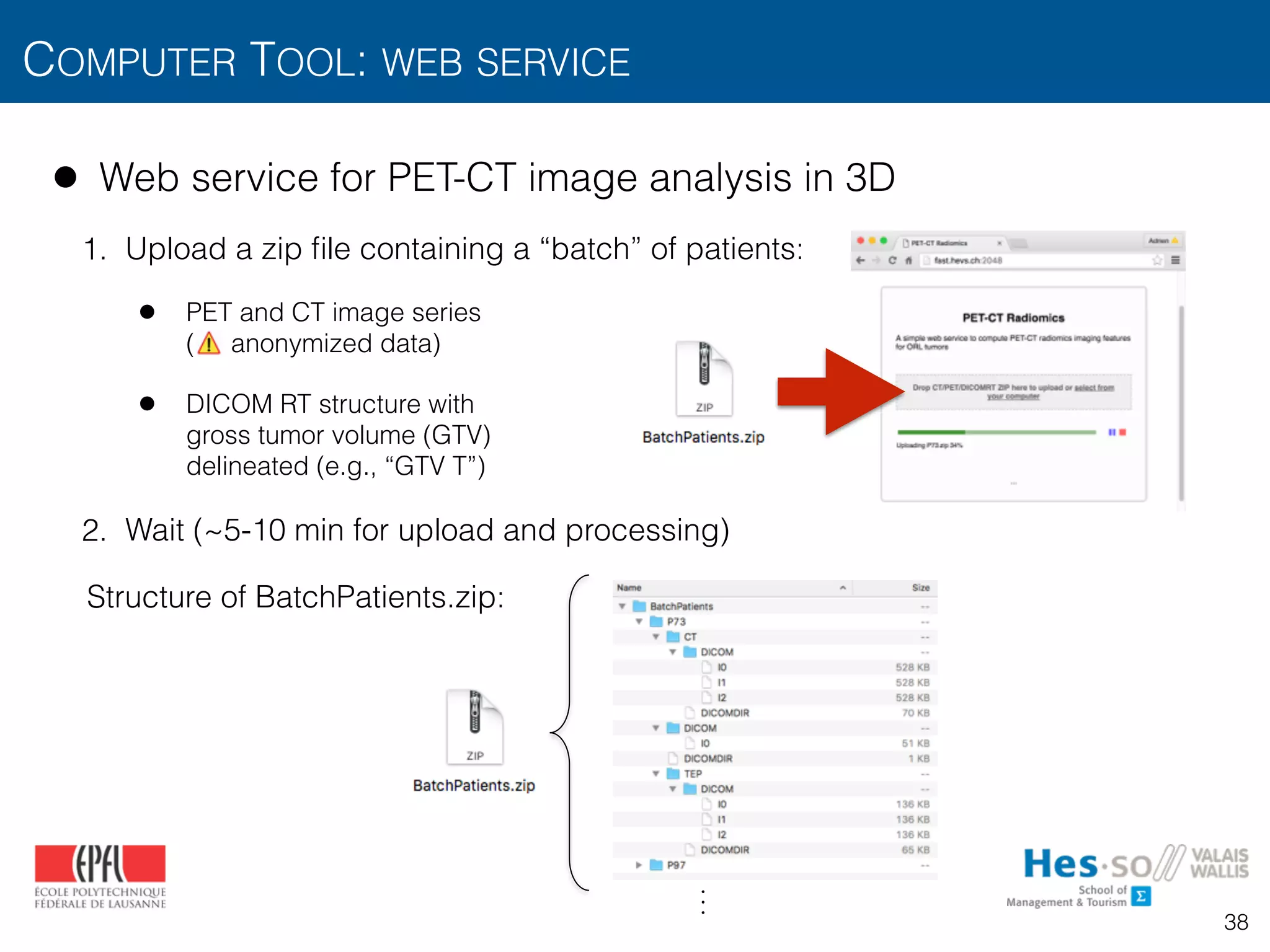
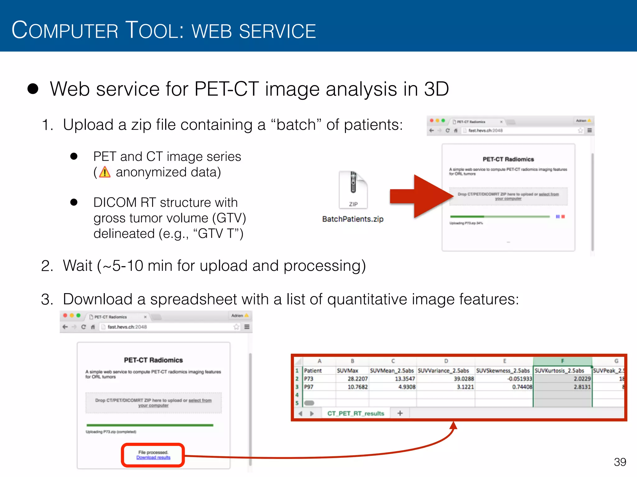
![• Web service for PET-CT image analysis in 3D
• Preprocessing
• PET-CT alignment, scale normalization with mm voxel size
• Intensity features from PET
• SUVmax, tumorVolume
• SUVmean, SUVvariance, SUVskewness, SUVkurtosis, SUVpeak, MTV, TLG
from multiple metabolic regions based on minimum SUV thresholds :
• Absolute (SUV):
• Relative to SUVmax (%):
• Intensity features from CT
• HUmean for , (SUV) et (SUVmax)
COMPUTER TOOL: WEB SERVICE
40
0.75 ⇥ 0.75 ⇥ 0.75
p
. . . . . .
2.5 5 8
p 2 [2.5 : 0.5 : 8]
p 2 [30 35 40 : 2 : 60 65 70]
Mp
M2.5 M5 M8
p = 3 p = 42%Mp](https://image.slidesharecdn.com/btaradiomics29-160819072138/75/A-3-D-Riesz-Covariance-Texture-Model-for-the-Prediction-of-Nodule-Recurrence-in-Lung-CT-40-2048.jpg)
![@
@x
@
@y
@
@z
• Web service for PET-CT image analysis in 3D
• 3D texture from PET and CT
• 3D LoG with scales
• 3D 1st-order Riesz (i.e., aligned gradients) with 4 dyadic scales
• 3D GLCMs with and averaged over all directions
(i.e., rotation-invariant)
• 11 GLCM features (see [Haralick1973, Soh1999, Clausi2002] for definitions):
Contrast, correlation, energy, homogeneity, entropy, InverseDiffMoment, SumAverage,
SumEntropy, SumVariance, DiffVariance, DiffEntropy
COMPUTER TOOL: WEB SERVICE
41
Table 3
Comparison of the various techniques used for 3-D biomedical texture analysis.
Technique Example of primitive Primitive neighborhood Illumination invariance Typical coverage of 3-D directions
GLCMs Voxel pairs No Incomplete for R > 1
RLE Linear No Incomplete for R > 1
scale 1 scale 2
LoG = 0.25 : 0.5 : 2.25
. . .
. . .
Mmargin
Mtexture
012,Depeursinge2015]
mage derivatives
een voxel values
41
terize the morphological properties of lung tissue associated with
tial lung diseases.16,17,20,21
They consist in counting the co-
ence of voxels with identical gray level values that are separated
stance d, which results in a co-occurrence matrix. Eleven statistics
xtracted from these matrices29
as texture attributes. The choices
d the number of gray levels were optimized by considering values
; 3} and {8, 16, 32}, respectively. The size of the vector of attri-
l was 540 for the gray-level histogram attributes (called HU there-
) and 396 for the GLCM attributes.
RESULTS
A leave-one-patient-out cross-validation evaluation was used to
te the performance of the proposed approach. The leave-one-
-out cross-validation consisted of using all patients but 1 to train
VM model and to measure the prediction performance on the re-
g test patient. The prediction performance was then averaged
ll possible combinations of training and test patients. Receiver
ng characteristic (ROC) curves of the system's performance in
ying between classic and atypical UIP are shown in Figure 4 for
nt feature groups and their combinations. The ROC curves were
ed by varying the decision threshold between the minimum and
ions X, Y, Z and 3 diagonals XY, XZ, and YZ. Figure 2 can be viewed
www.investigativeradiology.com 3
d reproduction of this article is prohibited.
y
@2
@x@z
@2
@y@z
scale 2
dGLCM = 1](https://image.slidesharecdn.com/btaradiomics29-160819072138/75/A-3-D-Riesz-Covariance-Texture-Model-for-the-Prediction-of-Nodule-Recurrence-in-Lung-CT-41-2048.jpg)
![• Web service for PET-CT image analysis in 3D
• 2 measures of metastasis spread [Fried2016]
• : distance between the primary tumor and the
barycenter of the metastases (TNdistance)
• : sum of distances between each metastasis and the
barycenter of the metastases (MetSpread)
COMPUTER TOOL: WEB SERVICE
42
kT
k ¯M
dT M
dTM = ||kT k ¯M ||
dMet =
X
i
||kMi
k ¯M ||
kM1
kM2](https://image.slidesharecdn.com/btaradiomics29-160819072138/75/A-3-D-Riesz-Covariance-Texture-Model-for-the-Prediction-of-Nodule-Recurrence-in-Lung-CT-42-2048.jpg)
![REFERENCES (SORTING IN ALPHABETICAL ORDER)
45
[Aerts2014] Aerts, H. J. W. L.; Velazquez, E. R.; Leijenaar, R. T. H.; Parmar, C.; Grossmann, P.; Carvalho, S.; Bussink, J.; Monshouwer, R.; Haibe-Kains, B.;
Rietveld, D.; Hoebers, F.; Rietbergen, M. M.; Leemans, C. R.; Dekker, A.; Quackenbush, J.; Gillies, R. J. & Lambin, P.
Decoding Tumour Phenotype by Noninvasive Imaging Using a Quantitative Radiomics Approach
Nature Communications, Nature Publishing Group, a division of Macmillan Publishers Limited. All Rights Reserved, 2014, 5
[Arsigny2006] Arsigny, V.; Fillard, P.; Pennec, X. & Ayache, N.
Log-Euclidean metrics for fast and simple calculus on diffusion tensors
Magnetic Resonance in Medicine, 2006, 56, 411-421
[Chenouard2011] Chenouard, N. & Unser, M.
3D Steerable Wavelets and Monogenic Analysis for Bioimaging
2011 IEEE International Symposium on Biomedical Imaging: From Nano to Macro, 2011, 2132-2135
[Chenouard2012] Chenouard, N. & Unser, M.
3D Steerable Wavelets in Practice
IEEE Transactions on Image Processing, 2012, 21, 4522-4533
[Cirujeda2015] Cirujeda, P.; Dicente Cid, Y.; Mateo, X. & Binefa, X.
A 3D Scene Registration Method via Covariance Descriptors and an Evolutionary Stable Strategy Game Theory Solver
International Journal of Computer Vision, 2015, 115, 306-329
[Cortes1995] Cortes, C. & Vapnik, V.
Support-vector networks
Machine learning, Springer, 1995, 20, 273-297
[Depeursinge2014] Depeursinge, A.; Foncubierta-Rodrguez, A.; Van De Ville, D. & Müller, H.
Three-dimensional solid texture analysis and retrieval in biomedical imaging: review and opportunities
Medical Image Analysis, 2014, 18, 176-196
[Depeursinge2015] Depeursinge, A.; Yanagawa, M.; Leung, A. N. & Rubin, D. L.
Predicting Adenocarcinoma Recurrence Using Computational Texture Models of Nodule Components in Lung CT
Medical Physics, 2015, 42, 2054-2063
[Förstner2003] Förstner, W. & Moonen, B.
A metric for covariance matrices
Geodesy - The Challenge of the 3rd Millennium, Springer, 2003, 299-309](https://image.slidesharecdn.com/btaradiomics29-160819072138/75/A-3-D-Riesz-Covariance-Texture-Model-for-the-Prediction-of-Nodule-Recurrence-in-Lung-CT-45-2048.jpg)
![REFERENCES (SORTING IN ALPHABETICAL ORDER)
46
[Gatenby2013] Gatenby, R. A.; Grove, O. & Gillies, R. J.
Quantitative Imaging in Cancer Evolution and Ecology
Radiology, 2013, 269, 8-14
[Ganeshan2013] Ganeshan, B.; Goh, V.; Mandeville, H. C.; Ng, Q. S.; Hoskin, P. J. & Miles, K. A.
Non-Small Cell Lung Cancer: Histopathologic Correlates for Texture Parameters at CT
Radiology, 2013, 266, 326-336
[Gevaert2012] Gevaert, O.; Xu, J.; Hoang, C. D.; Leung, A. N.; Xu, Y.; Quon, A.; Rubin, D. L.; Napel, S. & Plevritis, S. K. Non--Small Cell Lung Cancer:
Identifying Prognostic Imaging Biomarkers by Leveraging Public Gene Expression Microarray Data --- Methods and Preliminary Results
Radiology, 2012, 264, 387-396
[Karcher1977 Karcher, H.
Riemannian center of mass and mollifier smoothing
Communications on Pure and Applied Mathematics, 1977, 30, 509-541
[Mattonen2014] Mattonen, S. A.; Palma, D. A.; Haasbeek, C. J. A.; Senan, S. & Ward, A. D.
Early prediction of tumor recurrence based on CT texture changes after stereotactic ablative radiotherapy (SABR) for lung cancer
Medical Physics, 2014, 41, 1-14
[Moakher2005] Moakher, M.
A differential geometric approach to the geometric mean of symmetric positive-definite matrices
SIAM Journal on Matrix Analysis and Applications, 2005, 26, 735-747
[Pennec2006] Pennec, X.; Fillard, P. & Ayache, N.
A Riemannian framework for tensor computing
International Journal of Computer Vision, Springer, 2006, 66, 41-66
[Ravanelli2013] Ravanelli, M.; Farina, D.; Morassi, M.; Roca, E.; Cavalleri, G.; Tassi, G. & Maroldi, R.
Texture analysis of advanced non-small cell lung cancer (NSCLC) on contrast-enhanced computed tomography: prediction of the response to
the first-line chemotherapy European
Radiology, 2013, 23, 3450-3455
[Skibbe2012] Skibbe, H.; Reisert, M.; Schmidt, T.; Brox, T.; Ronneberger, O. & Burkhardt, H.
Fast Rotation Invariant 3D Feature Computation Utilizing Efficient Local Neighborhood Operators
IEEE Transactions on Pattern Analysis and Machine Intelligence, 2012, 34, 1563-1575
[Unser2011] Unser, M.; Chenouard, N. & Van De Ville, D.
Steerable Pyramids and Tight Wavelet Frames in
IEEE Transactions on Image Processing, 2011, 20, 2705-2721
[Ward2014] Ward, J. & Unser, M.
Harmonic Singular Integrals and Steerable Wavelets in
Applied and Computational Harmonic Analysis, 2014, 36, 183-197
L2(Rd
)
L2(Rd
)](https://image.slidesharecdn.com/btaradiomics29-160819072138/75/A-3-D-Riesz-Covariance-Texture-Model-for-the-Prediction-of-Nodule-Recurrence-in-Lung-CT-46-2048.jpg)

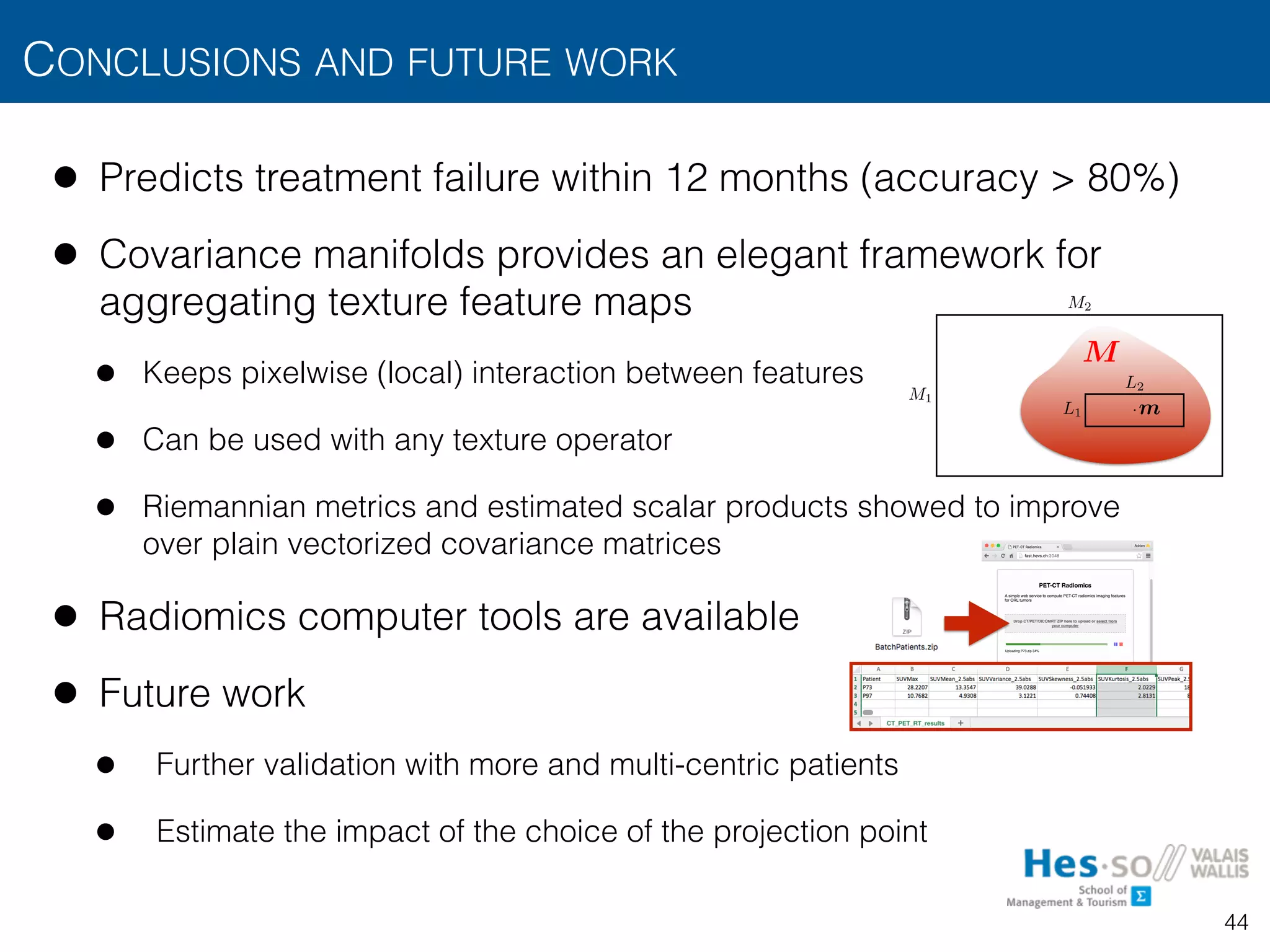
The document discusses a 3-dimensional Riesz-covariance texture model designed to predict nodule recurrence in lung CT scans. It highlights the use of locally aligned 3-D Riesz wavelets as texture operators along with Riemannian manifolds for efficient classification via support vector machines. The overall goal is to enable non-invasive personalized estimations of cancer treatment success based on detailed image analysis.


![Social media research in the health domain (tutorial) - [part 1]](https://cdn.slidesharecdn.com/ss_thumbnails/socialmediaresearchinthehealthdomain-short-170218080943-thumbnail.jpg?width=640&height=640&fit=bounds)