Downloaded 85 times


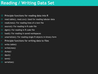
![Data Types
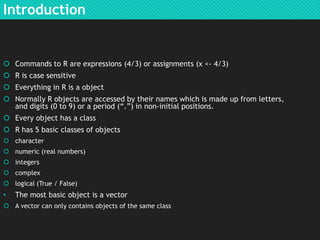
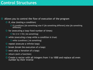
Matrix: vectors with dimension attribute. Dimension itself is an
integer vector of length 2 (nrow, ncol). Matrices are constructed
column wise.
m <- matrix(nrow=2, ncol=3)
m <- matrix(1:6, nrow=2, ncol=3)
x <- 1:3
y <- 10:12
cbind(x, y)
rbind(x,y)
Data frames (data.frame())
https://stat.ethz.ch/pipermail/rhelp/attachments/20101027/05a229bb/attachment.pl
Factors: Used for categorical data i.e. Male & Female or analyst,
senior analyst, manager etc.
x <- factor(c(“a”, “b”, “b”, “c”, “c”, “c”, “d”))
levels()
unclass(x)
levels([4:6])
Levels([4:6, drop=TRUE])](https://image.slidesharecdn.com/rlanguageintroduction-140121125601-phpapp01/85/R-language-introduction-10-320.jpg)
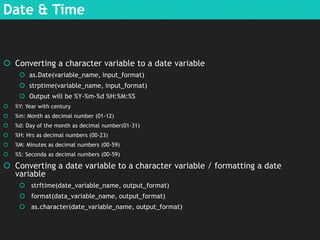
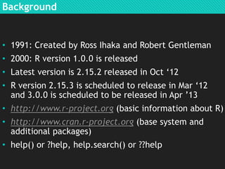
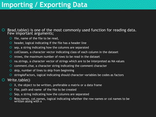
![Some Examples
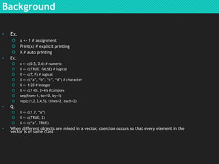
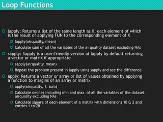
x <- c(“a”, “b”, “c”, “c”, “d”, “a”)
x[1], x[1:4], x[x > “a”], u <- x >”a”
x <- matrix(1:6,2,3)
x[1,2], x[1,], x[,1], x[1,2, drop=FALSE]
x <- list(var_1=c(1:10), var_2=c(“a”, “b”, “c”), var_3=0.6)
x[1], x[[1]], x$var_1
name <- “var_1”, x[name], x[[name]], x$name
x[c(1,3)], x[[c(1,3)]], x[[1]][[3]]
Produce a character vector containing var_1, var_2, var_3… var_999
Remove missing values from x <- c(1, 2, 3, NA, 4, 5, NA, 6)
y <- c(“a”, “b”, NA, NA, “c”, “d”, “e”, “f”), prepare a matrix containing
two columns x & y and does not have any missing value
What is the sum & mean of Wind for the observations which has
temperature greater then 60 & month equals to 5
How to create a new directory with a given name](https://image.slidesharecdn.com/rlanguageintroduction-140121125601-phpapp01/85/R-language-introduction-14-320.jpg)

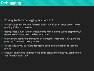


- R is a free software environment for statistical computing and graphics. It has an active user community and supports graphical capabilities. - R can import and export data, perform data manipulation and summaries. It provides various plotting functions and control structures to control program flow. - Debugging tools in R include traceback, debug, browser and trace which help identify and fix issues in functions.


![[1062BPY12001] Data analysis with R / week 2](https://cdn.slidesharecdn.com/ss_thumbnails/dataanalyzer01-180307063046-thumbnail.jpg?width=640&height=640&fit=bounds)