Response spectra

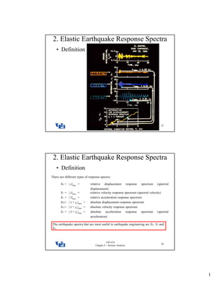
1
2. Elastic Earthquake Response Spectra
• Definition
CIE 619
Chapter 4 – Seismic Analysis
25
• Definition
There are different types of response spectra:
SD = |x| max = relative displacement response spectrum (spectral|| max p p p ( p
displacement)
SV = |x| max
 = relative velocity response spectrum (spectral velocity)
SA = |x| max
 = relative acceleration response spectrum
SDa= |x+x| s max = absolute displacement response spectrum
SVa= |x+x| s max = absolute velocity response spectrum
SA = |x+x| s max = absolute acceleration response spectrum (spectral
acceleration)
CIE 619
26
)
The earthquake spectra that are most useful in earthquake engineering are SD, SV and
SA.

2
• Definition
Northridge-Rinaldi
CIE 619
27
• Properties of Response Spectra
Response spectra have the following properties :
1 they give the maximum response values of a SDOF system subjected to a given1. they give the maximum response values of a SDOF system subjected to a given
earthquake accelerogram;
2. they give the maximum response values in each mode of a MDOF system
subjected to a given earthquake accelerogram; This result will be discussed
further in this chapter.
3. they indicate the frequency distribution of the seismic energy of a given
earthquake accelerogram, meaning that the response of a SDOF system is
CIE 619
28
q g , g p y
amplified when the seismic energy is close to its natural frequency.

3
• Exact Response Spectra
The relative displacement response spectrum is obtained directly by Duhamel’s integral
given by equation 4.69 :
|d)-(te)(x
1
-|=|x|=S d
)-(t-
s
t
0d
D maxmax sin 



The acceleration and the relative velocity are as follows :
dt
dx(t)
=(t)x
CIE 619
29
dt
x(t)d
=(t)x 2
2

By convolution, if a time function, F(t), is given by :
(t)
then its time derivative becomes :
 d)(t,f=F(t)
(t)u
(t)u
1
0

t)(t),u(f
dt
(t)du
-t)(t),u(f
dt
(t)du
+d
t
)(t,f
=
dt
dF(t)
0
0
1
1
(t)u
(t)u
1
0





CIE 619
30
(t)u0
the above is known also as Leibnitz derivative of an integrated function

4
Applying convolution to Duhamel’s integral given by equation 4.69, we have :
)-(te)(x
1
-=)(t,f d
)-(t-
s
d


 
sin



d)-(te)(x
1
-=x(t) d
)-(t-
s
t
0d
sin
t=(t)u
0=(t)u
1
0
The relative velocity is then :
 
d)-(te)(x-=(t)x d
)-(t-
s
t
0
cos 
(4 100)
t)(t),u(f
dt
(t)du
-t)(t),u(f
dt
(t)du
+d
t
)(t,f
=
dt
dF(t)
0
0
1
1
(t)u
(t)u
1
0





CIE 619
31
The relative velocity response spectrum is given by :


 
d)-(te)(x
-1
+ d
)-(t-
s
t
0
2
sin
|(t)x|=SV max

(4.100)
Similarly, the relative acceleration is obtained by differentiating equation 4.100 with
respect to time :
(t)x-d)-(te)(x
-1
)2-(1
+
d)-(te)(x2=(t)x
sd
)-(t-
s
t
0
2
2
d
)-(t-
t
0








sin
cos


(4.102)
CIE 619
32
The absolute acceleration response spectrum is then :
|(t)x+(t)x|=S sA max

5
CIE 619
33
Datafile
• Pseudo Response Spectra
Usually, a civil engineering structure has low damping (lower than 20% critical). The
following hypotheses can then be made :g yp
)(t-sinbyreplacedbecancos d 


)-(t
0,
d
d
2



CIE 619
34

6
• Pseudo Response Spectra
With these assumptions, equation 4.100 becomes:
x(t)=d)-(tex-(t)x d
)-(t-
s
t

sin 
 
d)-(te)(x-=(t)x d
)-(t-
s
t
0
cos 
(4.106)
The pseudo relative velocity response spectrum is then:
With the same assumptions, equation 4.102 is written:
( ))(ex( ) ds
0

S=S DV 
2)(t
t




 
d)-(te)(x
-1
+ d
)-(t-
s
t
0
2
sin
d)-(te)(x2=(t)x d
)-(t-
t
0
  
cos



d)-(te)(x
1
-=x(t) d
)-(t-
s
t
0d
sin
CIE 619
35
The pseudo absolute acceleration response spectrum becomes:
x(t)=d)-(texx+x 2
d
)-(t-
s
0
s  
sin 
S=S=S VD
2
A 
(t)x-d)-(te)(x
-1
)2-(1
+ sd
)-(t-
s
t
0
2
2
 

 
sin
(4.108)
• Comparison Between Exact and
Pseudo Response Spectra
– Comparing exact response spectra
(equations 4.100, 4.102) with pseudo
response spectra (equations. 4.106,
4.108) for different accelerograms,
yields the following tendencies:yields the following tendencies:
• in a system with zero damping,
results are essentially identical for
natural periods less than one second
(T < 1 s);
• when damping increases to 20 %
critical, differences are within 20 %
but without any observable bias;
• pseudo acceleration response
spectrum more precise than pseudo
velocity response spectrum.
CIE 619
36
– Variations within acceptable range
expected from seismic analysis.
– Pseudo response spectra must not be
used for highly damped systems ( >
20 % critical) or for systems with
long natural periods (T >> 1 s).

7
• Tripartite Representation
of Pseudo Response
Spectra
– In practice, responsep , p
spectra represented by a
graph with multiple
logarithmic scales called a
tripartite graph.
– Tripartite graph display on
same curve the following
information :
CIE 619
37
information :
• exact relative displacement
response spectrum;
• pseudo relative velocity
response spectrum;
• pseudo absolute acceleration
response spectrum.
• Tripartite Representation of Pseudo Response Spectra
– To understand tripartite graph, consider variation of
log10Sv with log10T for constant values of SA or SD.
a) SA = constant = C1
If the pseudo acceleration response spectrum is equal to a constant, C1, it can be
written:
operating with the log10 on this equation, it yields:
  S
T
2
=S=S=C=S VDD
2
1A


CIE 619
38
or
S+T-2=C V101010110 loglogloglog 
 2-C+T=S 1011010V10 loglogloglog

8
 2-C+T=S 1011010V10 loglogloglog
then
This result indicates that a line at + 45º on the tripartite graph represents a constant
spectral acceleration, SA .
 
 
1+=
Td
Sd
10
V10
log
log
CIE 619
39
b) SD = constant = C2
If the relative displacement response spectrum is equal to a constant, C2, it can bep p p q
written:
S
2
T
=
S
=C=S V
V
2D

operating with the log10 on this equation, it yields :
S+2-T=C V101010210 loglogloglog 
CIE 619
40
or
 2+C+T-=S 1021010V10 loglogloglog

9
then
 2+C+T-=S 1021010V10 loglogloglog
then
This result indicates that a line at -45º on a tripartite graph represents a constant
relative displacement spectrum, SD.
 
 
1-=
Td
Sd
10
V10
log
log
CIE 619
41
• Tripartite Representation of Pseudo
Response Spectra
– Figure illustrates, for different damping
values, response spectra of El Centro
earthquake (1940 05 18, comp. S00E).
– Response spectrum of an earthquake
er irreg larvery irregular.
– Spectrum has a general trapezoidal
shape (shape of a tent) characteristic of
earthquake response spectra and has
the following physical explanation :
• for long natural periods, maximum
relative displacement equal to
maximum ground displacement and
maximum absolute acceleration tends
toward zero;
• for intermediate natural periods
CIE 619
42
for intermediate natural periods,
relative displacement, relative velocity
and absolute acceleration amplified;
• for short natural periods, maximum
absolute acceleration equal to
maximum ground acceleration and
maximum relative displacement tends
toward zero.

10
• Simplified Design Response Spectra
– Motivation
• For practical seismic design of structures, simplified response
spectra are used.
• Different regions of simplified spectra represented by straight
lines.
• Position of these lines (amplitude) function of seismic hazard
of the region.
• Many simplified design response spectra have been proposed.
CIE 619
43
y p g p p p p
• Most common are described in the following sections.
– Housner’s Response Spectra (1959)
Relying on response spectra obtained for four historical earthquakes of Southern
California (El Centro, 1934, M=6.5; El Centro, 1940, M=6.7 and Tehachapi, 1952,
M=7.7) and one from Washington (Olympia, 1949, M=7.1)., G. Housner (1959)
proposed, for the first time, an “average design spectrum”. This spectrum was
calibrated for a maximum ground acceleration of 0,20g and for a probability of
exceedence of 50 %, in other words, for the average of the historical spectral values.
The values obtained from this spectrum are to be multiplied by a scale factor to take
into account the seismic hazard of the region. For example, if the design earthquake of
a given site is 0,15g, then the spectral acceleration will be:
CIE 619
44
HousnerofSof
20
15
equals A





SA

11
– Housner’s Response Spectra (1959)
CIE 619
45
– Newmark and Hall’s Response Spectra (1969)
• Developed for nuclear industry
• Simplified spectra based on standard ground motion
parameters:
– maximum ground acceleration : 0,50 g;
– maximum ground velocity : 61 cm/s (24 in/s);
– maximum ground displacement : 46 cm (18 in).
– Relying on the study of 28 earthquake records, values represent
l i b diff d i i
CIE 619
46
average relation between different ground seismic parameters.
– For a given site, values are scaled directly to the maximum design
acceleration, which is function of seismic hazard of the region.
– Simplified spectrum obtained by multiplying each branch of ground
parameters by an amplification factor which depends on damping
coefficient of the structure.

12
CIE 619
47
Note!
Table 4.2 Amplification factors for Newmark and Hall’s design response spectra
(From Newmark et Hall, 1982).
Damping ratio
% of critical
Probability of exceedence
of 16 %
(mean + 1 standard deviation)
Probability of exceedence of 50 %
(mean value)
SA SV SD SA SV SD
0,5 5,10 3,84 3,04 3,68 2,59 2,01
1 4,38 3,38 2,73 3,21 2,31 1,82
2 3,66 2,92 2,42 2,74 2,03 1,63
3 3,24 2,64 2,24 2,46 1,86 1,52
5 2,71 2,30 2,01 2,12 1,65 1,39
CIE 619
48
7 2,36 2,08 1,85 1,89 1,51 1,29
10 1,99 1,84 1,69 1,64 1,37 1,20
20 1,26 1,37 1,38 1,17 1,08 1,01
For the seismic design of nuclear plants, Newmark and Hall recommended the use of
amplification factors corresponding to a probability of exceedence of 16 %.

13
• Procedure to plot Newmark’s simplified spectra
– Step 1 - Plot of the ground motion parameters
» Limits of ground motion parameters linked by straight lines:
maximum horizontal acceleration, maximum horizontal velocity
and maximum horizontal displacement.
» If maximum horizontal acceleration is only known parameter at
site, standard ground motion parameters can be used with
maximum design acceleration, e.g. if maximum design
CIE 619
49
acceleration of 0,33g, at site is only known parameter:
 
 
  cm30,36=cm46
0,50
0,33
=ntdisplacemeground
cm/s40,26=cm/s61
0,50
0,33
=velocityground
g0,33=g0,50
0,50
0,33
=onacceleratiground


















• Simplified Design Response
Spectra
– Newmark and Hall’s
Response Spectra (1969)
Table 4.3 Recommended Damping Values.
Strain Level
Types of structures and conditions % of Critical
Damping
Response Spectra (1969)
• Procedure to plot Newmark’s
simplified spectra
– Step 2 - Plot different regions
of spectrum
» Amplification factors,
shown in Table 4.2, used
to plot different regions
welded steel, prestressed concrete,
reinforced concrete with light
cracking 2 to 3
reinforced concrete with heavy
cracking 3 to 5
less than 50 % of
the elastic limit
bolted or rivetted steel, nailed or
bolted timber 5 to 7
welded steel, prestressed concrete
without complete loss of
prestressing 5 to 7
prestressed concrete with
prestressing loss 7 to 10
CIE 619
50
p g
of simplified spectrum.
» Table 4.3 shows
recommended damping
values to be used.
prestressing loss 7 to 10
reinforced concrete 7 to 10
bolted or rivetted steel, bolted
timber 10 to 15
close to or over the
elastic limit nailed timber 15 to 20

14
• Procedure to plot Newmark’s simplified spectra
– Step 3 - Modification of spectral limits for high frequencies
– Find corner frequency, 1, which links velocity branch to acceleration
branch.
– At frequency of about 41, start reducing linearly acceleration branch
of spectrum until reaching limit of peak ground acceleration for a
frequency of 101.
– Theoretically, displacement branch should also be modified for low
CIE 619
51
y, p
frequencies (lower than 0.1 Hz). But, as low frequencies have little
impact on Civil Engineering structures, modification can be omitted.
– Design Response Spectrum of ASCE 7-05
CIE 619
52

15
CIE 619
53
CIE 619
54

16
CIE 619
55
CIE 619
56

17
CIE 619
57
CIE 619
58

18
CIE 619
59
CIE 619
60

19
CIE 619
61
– Consider a seismic zone in Southern California on Site
Class B (rock)
 
 
H )f(
g.
T
g.g.S
g.g.S
.FF
g.Sg;.S
D
Ds
va
s
338120
60
20
6090
3
2
0151
3
2
01
9051
1
1








0.4
0.6
0.8
1
1.2
ctralAcceleration(g)
ASCE 7-05 Design Spectrum
Newmark-Hall Spectrum, 5%damping, PGA=0.40 g
CIE 619
62
Hz).f(orT
Hz).f(or.
g.
g.
T
Hz).f(or.
g.
g
.T
LL
os
oo
0830sec12
671sec600
01
60
338sec120
01
20













0
0.2
0 1 2 3 4 5
Period (sec)
Spec

1
• Floor Response Spectra
– Response spectra, discussed in previous sections, used to determine maximum
response of SDOF structure subjected to base motion.
– Similarly, maximum response of equipment, located in a building, can be
obtained using response spectrum corresponding to the floor where theg p p p g
equipment is located.
– Vibration of a complex building varies from storey to storey, creating,
therefore, a variation in the response spectra of the various floors.
– Traditional technique used to generate a floor response spectrum is, first, to
calculate historical horizontal acceleration of a floor and then use this
accelerogram to construct a response spectrum.
– If a simplified design response spectrum of a floor is to be constructed, the
procedure starts with an ensemble of accelerograms at the base and the
CIE 619
64
procedure starts with an ensemble of accelerograms at the base and the
resulting spectra are smoothened.
– Because of the large quantity of calculations required to generate a floor
response spectrum, approximate methods have been proposed (Singh, 1975,
Biggs and Roesset, 1970).
Generation of
Floor Motion Ensembles
Generation of
Floor Motion Ensembles
Floor Response Spectra
• Floor Response Spectra
Dynamic
Analysis
0
0.2
0.4
0.6
0.8
1
1.2
0 1 2 3 4 5
Period (sec)
SpectralAcceleration(g)
0
0.2
0.4
0.6
0.8
1
1.2
0 1 2 3 4 5
Period (sec)
CIE 619
65
Ground Motion Ensembles
(Ground Response Spectra)
Ground Motion Ensembles
Ground Response Spectra
Building
0
0.2
0.4
0.6
0.8
1
1.2
0 1 2 3 4 5
Period (sec)

Response spectra

Recommended

Recommended

More Related Content

What's hot

What's hot (20)

Viewers also liked

Viewers also liked (17)

Similar to Response spectra

Similar to Response spectra (20)

Recently uploaded

Recently uploaded (20)

Response spectra