Downloaded 290 times
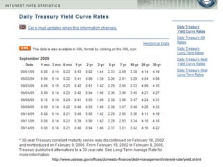

![Security Valuation with the APT:
An Example
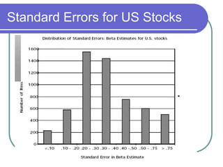
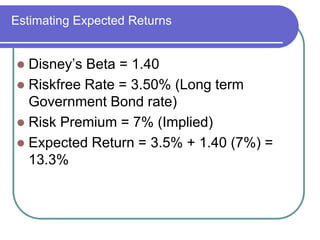
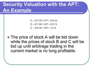
Riskless arbitrage
Requires no net wealth invested initially
Will bear no systematic or unsystematic risk but
Still earns a profit
Condition must be satisfied as follow:
1.
2
3
0i iw
0 iji ibw
0 ii i Rw i.e. actual portfolio return is positive
For all K factors [i.e. no systematic risk] and w is small
for all I [ unsystematic risk is fully diversified]
i.e. no net wealth invested
Wi the percentage investment in security i](https://image.slidesharecdn.com/chapter7-101031161331-phpapp02/85/Chapter-7-40-320.jpg)
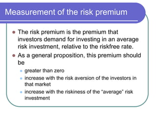
![Security Valuation with the APT:
An Example
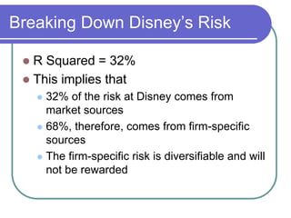
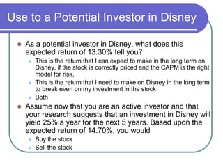
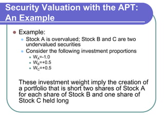
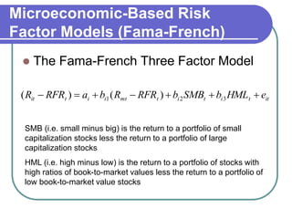
Net Initial Investment:
Short 2 shares of A: +70
Purchase 1 share of B: -35
Purchase 1 share of C: -35
Net investment: 0
Net Exposure to Risk Factors:
Factor 1 Factor 2
Weighted exposure from Stock A: (-1.0)(0.8) (-1.0)(0.9)
Weighted exposure from Stock B: (0.5)(-0.2) (0.5)(1.3)
Weighted exposure from Stock C: (0.5)(1.8) (0.5)(0.5)
Net risk exposure 0 0
Net Profit:
Stock A Stock B Stock C
[2(35)-2(37.20)]+[37.80-35]+[38.50-35] =$1.90](https://image.slidesharecdn.com/chapter7-101031161331-phpapp02/85/Chapter-7-42-320.jpg)

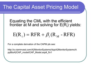
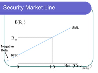
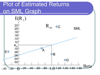
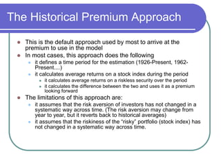
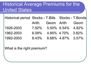
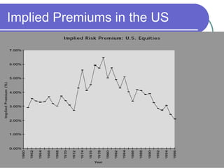
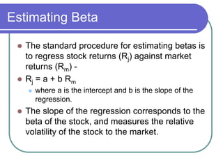
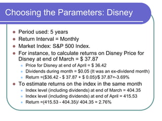
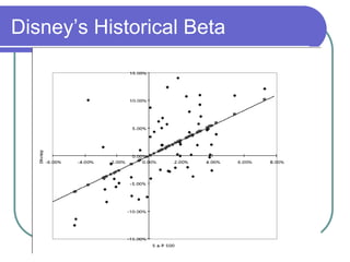
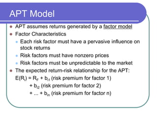
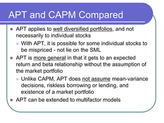
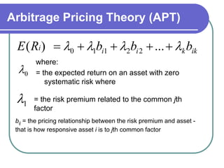
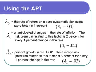
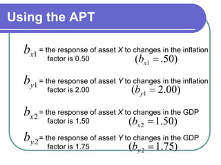
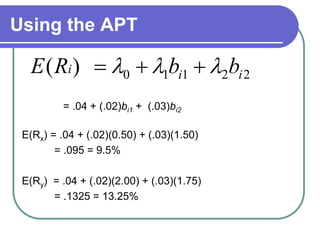
The Arbitrage Pricing Theory (APT) provides an alternative to the Capital Asset Pricing Model (CAPM) for estimating expected returns. The APT assumes returns are generated by multiple systematic risk factors rather than a single market factor. It allows for assets to be mispriced and does not require assumptions of a market portfolio or homogeneous expectations. Under the APT, the expected return of an asset is equal to the risk-free rate plus the product of each risk factor's premium and the asset's sensitivity to that factor.


