The turbidity (TB) varies with time and space in the reservoir

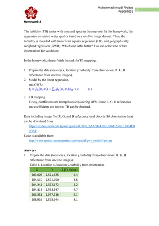
1. 1
Muhammad Irsyadi Firdaus
P66067055
Homework 3
The turbidity (TB) varies with time and space in the reservoir. In this homework, the
regression estimated water quality based on a satellite image dataset. Then, the
turbidity is modeled with linear least squares regression (LR), and geographically
weighted regression (GWR). Which one is the better? You can select one or two
observations for validation.
In the homework, please finish the task for TB mapping.
1. Prepare the data (location x, location y, turbidity from observation; R, G, B
reflectance from satellite images).
2. Model by the linear regression,
and GWR:
𝑌𝑖 = 𝛽0(𝑢𝑖, 𝑣𝑖) + ∑ 𝛽 𝑘(𝑢𝑖, 𝑣𝑖)𝑋𝑖𝑘 + 𝜀𝑖𝑘 (1)
3. TB mapping
Firstly, coefficients are interpolated considering IDW. Since R, G, B reflectance
and coefficients are known, TB can be obtained.
Data including image file (R, G, and B reflectance) and obs.xls (10 observation data)
can be download from
https://mybox.ncku.edu.tw/navigate/s/8C86FC7A82B2428BBBADA963E2434D0
9GSY
Code is available from:
http://www.spatial-econometrics.com/spatial/gwr_models/gwr.m
Answers
1. Prepare the data (location x, location y, turbidity from observation; R, G, B
reflectance from satellite images).
Table 1. Location x, location y, turbidity from observation
X Y Z (TB Value)
203,006 2,571,625 5.4
204,510 2,571,700 3.6
204,341 2,572,172 3.2
204,314 2,573,547 4.7
206,351 2,577,336 5.1
208,939 2,578,944 8.1

2. 2
Muhammad Irsyadi Firdaus
P66067055
208,258 2,578,681 5.4
206,745 2,575,800 4.6
204,854 2,574,015 2.7
202,857 2,571,566 4.4
 R, G, B reflectance from satellite images
To get RGB value and row column value, I use ENVI software. So get the
value as below.
Table 2. RGB value
Red Green Blue
1.1522 2.1010 1.1610
1.1522 2.1010 1.1259
1.1012 1.9714 1.1142
1.1012 2.0038 1.1259
1.1522 2.1334 1.1610
1.3817 2.5870 1.3131
1.2542 2.3926 1.2546
1.1522 2.1334 1.1376
1.1012 2.0038 1.1259
1.1777 2.0686 1.1727
Table 3. Row and Column Value
Column Row
888 4837
1640 4800
1555 4564
1542 3876
2560 1982
3854 1178
3514 1309
2. Model by the linear regression, and GWR
Geographically weighted regression (GWR) is an exploratory technique
mainly intended to indicate where non-stationarity is taking place on the map, that
is where locally weighted regression coefficients move away from their global
values. On the linear regression model using 10 point samples and obtained linear
parameters as in the table below.
Code Linear Regression using MatLAB

3. 3
Muhammad Irsyadi Firdaus
P66067055
Tabel 4. Linear Parameters
𝜷 𝟎 -14.8214548000326
𝜷 𝟏 7.31199506006149
𝜷 𝟐 1.15664710908197
𝜷 𝟑 7.25380884793830
Tabel 5. Result of regression linear model
Points
Turbidity Value
(Linear Regression)
TB
Observation
The difference
point value
1 4.45521355680786 5.4 0.944786443
2 4.20060486624522 3.6 0.600604866
3 3.59292208932419 3.2 0.392922089
4 3.71526701917932 4.7 0.984732981
5 4.49268892314211 5.1 0.607311077
6 7.79875124387722 8.1 0.301248756
7 6.21727185810946 5.4 0.817271858
8 4.32294979610036 4.6 0.277050204
9 3.71526701917932 2.7 1.015267019
10 4.68906362802605 4.4 0.289063628
Geographically Weighted Regression (GWR) Model
Y = 𝛽0 + 𝛽1 ∗ R + 𝛽2 ∗ G + 𝛽3 ∗ B + Residual
Or

4. 4
Muhammad Irsyadi Firdaus
P66067055
𝑌𝑖 = 𝛽0(𝑢𝑖, 𝑣𝑖) + ∑ 𝛽 𝑘(𝑢𝑖, 𝑣𝑖)𝑋𝑖𝑘 + 𝜀𝑖
𝑘
Code GWR Parameters using MatLAB
Table 6. Beta values on each points
Number Residual
1 -17.7586 -4.7319 3.2761 17.9845 0.8475
2 -17.9070 -4.9393 3.3681 18.1482 -0.3114
3 -17.7966 -4.7354 3.3677 17.8495 -0.3159
4 -17.8423 -5.2326 3.7392 17.7107 0.8712
5 -11.4069 16.4338 0.4352 -3.4458 0.6439
6 -12.0015 17.6359 -0.2099 -2.9730 0.1810
7 -11.9806 17.3069 -0.1089 -2.8454 -0.4950
8 -11.7158 12.6489 1.6192 -1.5858 0.0913
9 -17.5399 -4.68864 3.9779 16.4639 -1.1046
10 -17.797119 -4.8620 3.2949 18.1144 -0.1356
Table 7. Result of GWR regression model
Number Turbidity Value
(GWR Regression)
TB
Observation
1
5.400 5.4
2
3.600 3.6
3
3.200 3.2
4
4.700 4.7
5
5.100 5.1

5. 5
Muhammad Irsyadi Firdaus
P66067055
6
8.100 8.1
7
5.400 5.4
8
4.600 4.6
9
2.700 2.7
10
4.400 4.4
The turbidity is modeled with linear least squares regression (LR), and
geographically weighted regression (GWR). After comparing the results between linear
least squares regression (table 5) and geographically weighted regression (GWR)
results in Table 7, the best result for calculating the turbidity (TB) varies is the
geographically weighted regression (GWR) method because it has the same value as
TB Observation.
3. Turbidity Mapping
Code Turbidity Mapping using MatLAB
IMGBlue = imread('D:My DataSemester 1Spatial Enviromental Data
Analysis And ModelHW320090903BLUE_20090903_RN_Tiff.tif');
IMGGreen = imread('D:My DataSemester 1Spatial Enviromental Data
Analysis And ModelHW320090903GREEN_20090903_RN_Tiff.tif');
IMGRed = imread('D:My DataSemester 1Spatial Enviromental Data
Analysis And ModelHW320090903Red_20090903_RN_Tiff.tif');
TH = imread('D:My DataSemester 1Spatial Enviromental Data Analysis
And
ModelHW3NDWI_Mask_20090903NDWI_Mask_20090903NDWI_Mask_20090903_RN
_Tiff.tif');
SX=size(IMGBlue);
% Sampling
RGB1 = RGB(1:10,:);
XYZ1 = XYZ(1:10,:);
RowColumn1 = RowColumn(1:10,:);
% GWR
I = ones(10,1);
A(:,1) = I;
A(:,2) = RGB1(:,1);
A(:,3) = RGB1(:,2);
A(:,4) = RGB1(:,3);
res = gwr(XYZ1(:,3),A,RowColumn1(:,1),RowColumn1(:,2));

6. 6
Muhammad Irsyadi Firdaus
P66067055
% Parameters
Beta = res.beta;
Residual = res.resid;
% Cropping area
R = zeros(SX(1),SX(2));
G = zeros(SX(1),SX(2));
B = zeros(SX(1),SX(2));
for i =1:SX(1)
for j=1:SX(2)
if TH(i,j)==1
R(i,j)=IMGRed(i,j);
G(i,j)=IMGGreen(i,j);
B(i,j)=IMGBlue(i,j);
else
R(i,j)=0;
G(i,j)=0;
B(i,j)=0;
end
end
end
clear IMGRed IMGGreen IMGBlue
% IDW of Parameters
X1 = RowColumn(1:10,1);
Y1 = RowColumn(1:10,2);
Xu=zeros(SX(1),1);
Yu=zeros(SX(1),1);
for i = 1:SX(1)
Xu(i)=i;
Yu(i)=i;
end
IDWLamda = IDW(X1,Y1,Beta(:,1),Xu,Yu,3,'fr',9500);
IDWRed = IDW(X1,Y1,Beta(:,2),Xu,Yu,3,'fr',9500);
IDWGreen = IDW(X1,Y1,Beta(:,3),Xu,Yu,3,'fr',9500);
IDWBlue = IDW(X1,Y1,Beta(:,4),Xu,Yu,3,'fr',9500);
IDWResidual = IDW(X1,Y1,Residual(:,1),Xu,Yu,3,'fr',9500);
% Cropping area
IDW_R = zeros(SX(1),SX(2));
IDW_G = zeros(SX(1),SX(2));

7. 7
Muhammad Irsyadi Firdaus
P66067055
IDW_B = zeros(SX(1),SX(2));
IDW_Lamda = zeros(SX(1),SX(2));
IDW_Resid = zeros(SX(1),SX(2));
for i =1:SX(1)
for j=1:SX(2)
if TH(i,j)==1
IDW_R(i,j)=IDWRed(i,j);
IDW_G(i,j)=IDWGreen(i,j);
IDW_B(i,j)=IDWBlue(i,j);
IDW_Lamda(i,j)=IDWLamda(i,j);
IDW_Resid(i,j)=IDWResidual(i,j);
else
IDW_R(i,j)=0;
IDW_G(i,j)=0;
IDW_B(i,j)=0;
IDW_Lamda(i,j)=0;
IDW_Resid(i,j)=0;
end
end
end
% Data reshapping
RB_IDW = reshape(IDW_B,SX(1)*SX(2),1);
RG_IDW = reshape(IDW_G,SX(1)*SX(2),1);
RR_IDW = reshape(IDW_R,SX(1)*SX(2),1);
LL_IDW = reshape(IDW_Lamda,SX(1)*SX(2),1);
RES_IDW = reshape(IDW_Resid,SX(1)*SX(2),1);
% DATA RGB
RR = reshape(R,SX(1)*SX(2),1);
RG = reshape(G,SX(1)*SX(2),1);
RB = reshape(B,SX(1)*SX(2),1);
% Turbidity Mapping
for i=1:SX(1)*SX(2)
RTBgwr(i)=
LL_IDW(i,1)+(RR(i)*RR_IDW(i))+(RG(i)*RG_IDW(i))+(RB(i)*RB_IDW(i))+RES
_IDW(i);
end
RBgwr = reshape(RTBgwr,SX(1),SX(2));
image(RBgwr,'CDataMapping','scaled');

8. 8
Muhammad Irsyadi Firdaus
P66067055
colorbar;
Figure 1. Turbidity (Linear Regression) after applying IDW model in Matlab
Figure 2. Turbidity (GWR) after applying IDW model in Matlab