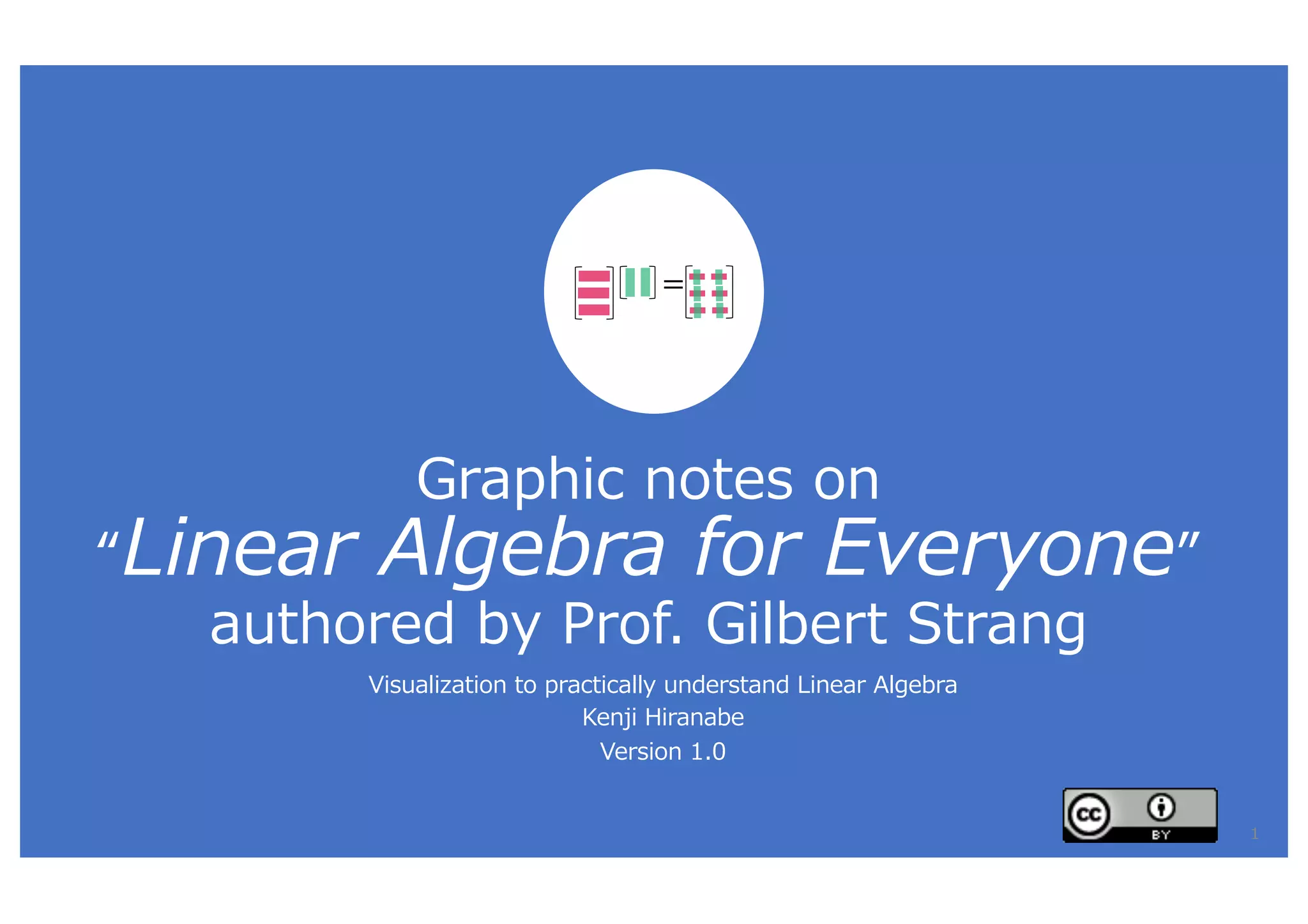
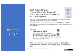
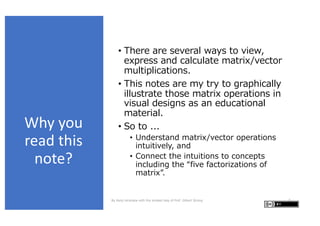
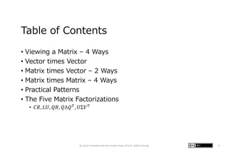
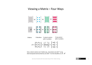
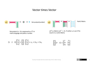
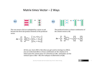
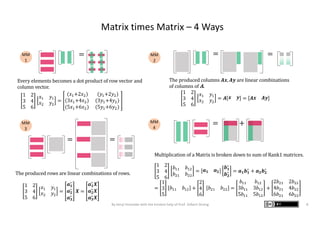
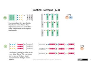
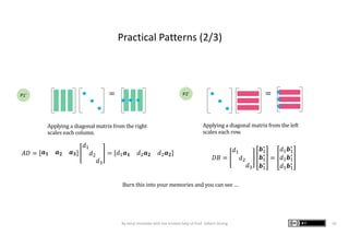
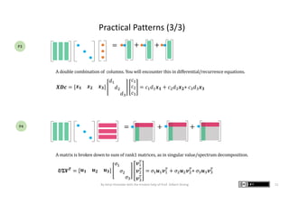
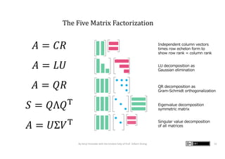
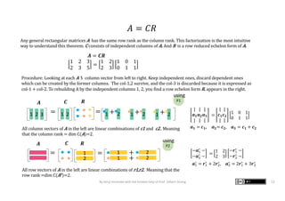
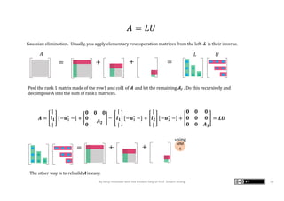
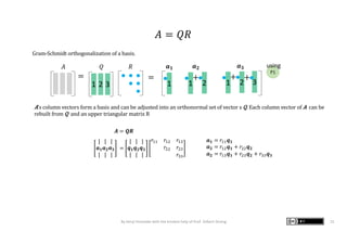
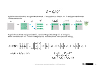
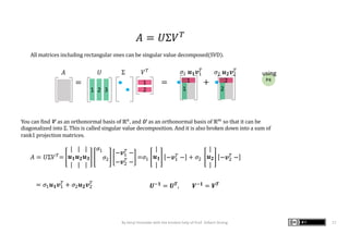
The document presents graphic notes summarizing Professor Gilbert Strang's book 'Linear Algebra for Everyone,' aimed at providing an intuitive understanding of linear algebra concepts through visual illustrations. It highlights key topics such as matrix operations, different multiplication methods, and various matrix factorizations including SVD. Additionally, it serves as an educational resource with links to complementary MIT course materials.

1. Graphic notes on
“Linear Algebra for Everyone”
authored by Prof. Gilbert Strang
Visualization to practically understand Linear Algebra
Kenji Hiranabe
Version 1.0
=
1

2. What is
this?
• Prof. Gilbert Strangʻs
“Linear Algebra for Everyone”
is a great book for an introduction
to Linear Algebra!
• Not theorem-proof chains but “matrix languages” and examples to get
intuitive understanding for practical applications.
• Linked to the best Linear Algebra course video MIT 18.06 and 18.065
youtube MIT OpenCourseWare playlist with over 2 milion subscribers(I am
one of them!)
• Hightlights…
• Four ways to AB=C
• The fundamental four subspaces.
• The five factorization of matrix.
• SVD as the climax, not Jordan block decoposition.
• Introduction to Data Science
• I tried to capture and convey the concepts in (1) and (2)
graphically and wanted to share design ideas for educational
use.
By Kenji Hiranabe with the kindest help of Prof. Gilbert Strang 2
1
2

3. Why you
read this
note?
• There are several ways to view,
express and calculate matrix/vector
multiplications.
• This notes are my try to graphically
illustrate those matrix operations in
visual designs as an educational
material.
• So to ...
• Understand matrix/vector operations
intuitively, and
• Connect the intuitions to concepts
including the “five factorizations of
matrix”.
By Kenji Hiranabe with the kindest help of Prof. Gilbert Strang 3

4. Table of Contents
• Viewing a Matrix – 4 Ways
• Vector times Vector
• Matrix times Vector – 2 Ways
• Matrix times Matrix – 4 Ways
• Practical Patterns
• The Five Matrix Factorizations
• 𝐶𝑅, 𝐿𝑈, 𝑄𝑅, 𝑄Λ𝑄!, 𝑈Σ𝑉!
By Kenji Hiranabe with the kindest help of Prof. Gilbert Strang 4

5. = = =
2 column vectors
with 2 numbers
3 row vectors
with 2 numbers
6 Numbers1 Matrix
Viewing a Matrix – Four Ways
𝐴 =
𝑎!! 𝑎!"
𝑎"! 𝑎""
𝑎#! 𝑎#"
=
|
𝒂 𝟏
|
|
𝒂 𝟐
|
=
−𝒂!
∗ −
−𝒂"
∗ −
−𝒂#
∗ −
Here, column vectors are in bold as 𝒂 𝟏, row vectors are with * as 𝒂"
∗
.
And transposed vectors/matrices are with T on the shoulders as 𝒂 𝑻, 𝑨 𝑻
𝐴 =
1 4
2 5
3 6
=
1 4
2 5
3 6
=
1 4
2 5
3 6
By Kenji Hiranabe with the kindest help of Prof. Gilbert Strang 5

6. = = =Dot product(number) Rank1 Matrix
v1 =
1
2
3
𝑥 𝑦 =
𝑥 𝑦
2𝑥 2𝑦
3𝑥 3𝑦
Vector times Vector
1 2 3
𝑥!
𝑥"
𝑥#
=
1
2
3
,
𝑥!
𝑥"
𝑥#
= 𝑥! + 2𝑥" + 3𝑥#
𝑎𝑏!
is a Matrix (𝑎𝑏!
= 𝐴). If neither 𝑎, 𝑏 are 0 The
result 𝐴 is a rank1 Matrix.
Dot product (𝑎 ) 𝑏) is expressed as 𝑎!
𝑏 in
matrix language and yields a number.
v2
By Kenji Hiranabe with the kindest help of Prof. Gilbert Strang 6

7. = = +
Matrix times Vector – 2 Ways
The row vectors of A are multiplied by a vector x and
become the three dot-product elements of the produced
vector.
The produced vector is a linear combination of
the column vectors of A.
𝑨𝒙 =
1 2
3 4
5 6
𝑥!
𝑥"
=
(𝑥!+2𝑥")
(3𝑥! + 4𝑥")
(5𝑥! + 6𝑥")
𝑨𝒙 =
1 2
3 4
5 6
𝑥!
𝑥"
= 𝑥!
1
3
5
+ 𝑥"
2
4
6
At first, you learn (Mv1). But when you get used to viewing it as (Mv2),
you can understand 𝑨𝒙 as a linear combination of the columns of A,
which spans the column space of A denoted as C 𝑨 , and further, see the
solution space of 𝑨𝒙 = 𝟎 as the nullspace of A denoted as N 𝑨 .
Mv1 Mv2
By Kenji Hiranabe with the kindest help of Prof. Gilbert Strang 7

8. Matrix times Matrix – 4 Ways
=
= +
1 2
3 4
5 6
𝑥" 𝑦"
𝑥# 𝑦#
=
(𝑥"+2𝑥#) (𝑦"+2𝑦#)
(3𝑥"+4𝑥#) (3𝑦"+4𝑦#)
(5𝑥"+6𝑥#) (5𝑦"+6𝑦#)
1 2
3 4
5 6
𝑥" 𝑦"
𝑥# 𝑦#
= 𝑨 𝒙 𝒚 = 𝑨 𝒙 𝑨𝒚
= =
= =
1 2
3 4
5 6
𝑏"" 𝑏"#
𝑏#" 𝑏##
= 𝒂 𝟏 𝒂 𝟐
𝒃 𝟏
∗
𝒃 𝟐
∗ = 𝒂 𝟏 𝒃 𝟏
∗
+ 𝒂 𝟐 𝒃 𝟐
∗
=
1
3
5
𝑏"" 𝑏"# +
2
4
6
𝑏#" 𝑏## =
𝑏"" 𝑏"#
3𝑏"" 3𝑏"#
5𝑏"" 5𝑏"#
+
2𝑏#" 2𝑏##
4𝑏#" 4𝑏##
6𝑏#" 6𝑏##
The produced columns 𝑨𝒙, 𝑨𝒚 are linear combinations
of columns of A.
1 2
3 4
5 6
𝑥" 𝑦"
𝑥# 𝑦#
=
𝒂 𝟏
∗
𝒂 𝟐
∗
𝒂 𝟑
∗
𝑿 =
𝒂 𝟏
∗
𝑿
𝒂 𝟐
∗
𝑿
𝒂 𝟑
∗
𝑿
Multiplication of a Matrix is broken down to sum of Rank1 matrices.
The produced rows are linear combinations of rows.
Every elements becomes a dot product of row vector and
column vector.
MM
1
MM
2
MM
3
MM
4
By Kenji Hiranabe with the kindest help of Prof. Gilbert Strang 8

9. Practical Patterns (1/3)
2 3
=
1 2 31 1
=
21
+
3
+
2
=
21
+
3
+
3
=
21
+
3
+
1
2
3
= 1
2
3
1 = +1 2 3+
2 = +1 2 3+
3 = +1 2 3+
MM
2
Mv2
MM
3
Operations from the right effect to
the columns of the Matrix. This
expression can be seen as the three
linear combinations in the right in
one formula.
P1
P2
using
using
By Kenji Hiranabe with the kindest help of Prof. Gilbert Strang 9
Operations from the left effect to the
rows of the Matrix. This expression
can be seen as the three linear
combinations in the right in one
formula.

10. = =
𝐴𝐷 = 𝒂 𝟏 𝒂 𝟐 𝒂 𝟑
𝑑!
𝑑"
𝑑#
= 𝑑! 𝒂 𝟏 𝑑" 𝒂 𝟐 𝑑" 𝒂 𝟐
𝐷𝐵 =
𝑑!
𝑑"
𝑑#
𝒃!
∗
𝒃!
∗
𝒃!
∗
=
𝑑! 𝒃!
∗
𝑑! 𝒃!
∗
𝑑! 𝒃!
∗
Applying a diagonal matrix from the right
scales each column.
Applying a diagonal matrix from the left
scales each row.
Burn this into your memories and you can see …
P1’ P2’
By Kenji Hiranabe with the kindest help of Prof. Gilbert Strang 10
Practical Patterns (2/3)

11. Practical Patterns (3/3)
= + +
A double combination of columns. You will encounter this in differential/recurrence equations.
=
𝑿𝑫𝒄 = 𝒙 𝟏 𝒙 𝟐 𝒙 𝟑
𝑑!
𝑑"
𝑑#
𝑐!
𝑐"
𝑐#
= 𝑐! 𝑑! 𝒙 𝟏 + 𝑐" 𝑑" 𝒙 𝟐+ 𝑐# 𝑑# 𝒙 𝟑
𝑼𝚺𝑽 𝑻 = 𝒖 𝟏 𝒖 𝟐 𝒖 𝟑
𝜎!
𝜎"
𝜎#
𝒗!
-
𝒗"
-
𝒗#
-
= 𝜎! 𝒖! 𝒗!
-
+ 𝜎" 𝒖" 𝒗"
-
+ 𝜎# 𝒖# 𝒗#
-
+ +
A matrix is broken down to sum of rank1 matrices, as in singular value/spectrum decomposition.
P3
P4
By Kenji Hiranabe with the kindest help of Prof. Gilbert Strang 11

12. The Five Matrix Factorization
𝐴 = 𝐶𝑅
𝐴 = 𝐿𝑈
𝐴 = 𝑄𝑅
𝑆 = 𝑄Λ𝑄!
𝐴 = 𝑈Σ𝑉!
By Kenji Hiranabe with the kindest help of Prof. Gilbert Strang 12
Independent column vectors
times row echelon form to
show row rank = column rank
LU decomposition as
Gaussian elimination
QR decomposition as
Gram-Schmidt orthogonalization
Eigenvalue decomposition
symmetric matrix
Singular value decomposition
of all matrices

13. 𝐴 = 𝐶𝑅
Procedure: Looking at each A ‘s column vector from left to right. Keep independent ones, discard dependent ones
which can be created by the former columns. The col-1,2 survive, and the col-3 is discarded because it is expressed as
col-1 + col-2. To rebuilding A by the independent columns 1, 2, you find a row echelon form R. appears in the right.
Any general rectangular matrices A has the same row rank as the column rank. This factorization is the most intuitive
way to understand this theorem. C consists of independent columns of A. And R is a row reduced echelon form of A.
2 =
1 2 3
2 3 5
=
1 2
2 3
1 0 1
0 1 1
1
|
𝒂 𝟏
|
|
𝒂 𝟐
|
|
𝒂 𝟑
|
=
|
𝒄 𝟏
|
|
𝒄 𝟐
|
1 0 1
0 1 1
𝒂 𝟏 = 𝒄 𝟏, 𝒂 𝟐= 𝒄 𝟐, 𝒂 𝟑 = 𝒄 𝟏 + 𝒄 𝟐
−𝒂"
∗
−
−𝒂#
∗
−
=
1 2
2 3
−𝒓"
∗
−
−𝒓#
∗
−
𝒂"
∗
= 𝒓"
∗
+ 2𝒓#
∗
, 𝒂#
∗
= 2𝒓"
∗
+ 3𝒓#
∗
213 = 1 + 2 1 + 2 1 + 2
All column vectors of A in the left are linear combinations of c1 and c2.. Meaning
that the column rank = dim C(A)=2.
= +1
2
1 2
1 2+
=
All row vectors of A in the left are linear combinations of r1,r2. Meaning that the
row rank =dim C(AT)=2.
𝑨 = 𝑪𝑹
P1
P2
using
using
By Kenji Hiranabe with the kindest help of Prof. Gilbert Strang 13
𝑨 𝑪 𝑹
𝑨 𝑪 𝑹

14. == + +
𝑨 =
|
𝒍 𝟏
|
−𝒖!
∗
− +
𝟎 𝟎 𝟎
𝟎
𝟎
𝑨 𝟐
＝
|
𝒍 𝟏
|
−𝒖!
∗
− +
|
𝒍 𝟐
|
−𝒖"
∗
− +
𝟎 𝟎 𝟎
𝟎 𝟎 𝟎
𝟎 𝟎 𝑨 𝟑
= 𝑳𝑼
𝐴 = 𝐿𝑈
Peel the rank 1 matrix made of the row1 and col1 of A and let the remaining A1 . Do this recursively and
decompose A into the sum of rank1 matrices.
= + +
The other way is to rebuild A is easy.
MM
4
Gaussian elimination. Usually, you apply elementary row operation matrices from the left. L is their inverse.
𝐿 𝑈
using
By Kenji Hiranabe with the kindest help of Prof. Gilbert Strang 14
𝐴

15. ==
𝐴 = 𝑄𝑅
A’s column vectors form a basis and can be adjusted into an orthonormal set of vector s Q. Each column vector of A can be
rebuilt from Q and an upper triangular matrix R
Gram-Schmidt orthogonalization of a basis.
2 31
|
𝒂 𝟏
|
|
𝒂 𝟐
|
|
𝒂 𝟑
|
=
|
𝒒 𝟏
|
|
𝒒 𝟐
|
|
𝒒 𝟑
|
𝑟"" 𝑟"# 𝑟"(
𝑟## 𝑟#(
𝑟((
31
+
1 2
+
1 2
+
𝒂 𝟏 = 𝑟"" 𝒒 𝟏
𝒂 𝟐 = 𝑟"# 𝒒 𝟏 + 𝑟## 𝒒 𝟐
𝒂 𝟐 = 𝑟"( 𝒒 𝟏 + 𝑟#( 𝒒 𝟐 + 𝑟(( 𝒒 𝟑
𝑨 = 𝑸𝑹
P1
using
By Kenji Hiranabe with the kindest help of Prof. Gilbert Strang 15
𝑄 𝑅𝐴 𝒂 𝟏 𝒂 𝟐 𝒂 𝟑

16. 𝑺 = 𝑸𝜦𝑸-=
|
𝒒 𝟏
|
|
𝒒 𝟐
|
|
𝒒 𝟑
|
𝜆!
𝜆"
𝜆#
−𝒒!
-
−
−𝒒"
- −
−𝒒#
- −
=𝜆!
|
𝒒 𝟏
|
−𝒒!
-
− + 𝜆"
|
𝒒 𝟐
|
−𝒒"
-
− + 𝜆#
|
𝒒 𝟑
|
−𝒒#
- −
𝑆 = 𝑄𝛬𝑄3
A symmetric matrix S is diagonalized into Λ by an orthogonal matrix Q and its transpose.
And it is broken down into a sum of rank1 projection matrices(known as the spectrum theory).
= 𝜆! 𝑷! + 𝜆" 𝑷 𝟐 + 𝜆# 𝑷 𝟑
Eigenvalue decomposition of a symmetric matrix S. All the eigenvalues are real, and all the eigenvectors can be
chosen orthonormal.
2 31
= + += 1
2
3
1
1
2
2
3
3
𝑺 = 𝑺 𝑻, 𝑸 𝑻 = 𝑸.𝟏
𝑷 𝟏
𝟐
= 𝑷 𝟐
𝟐
= 𝑷 𝟏
𝟐
= 𝑰
𝑷 𝟏 𝑷 𝟐 = 𝑷 𝟐 𝑷 𝟑 = 𝑷 𝟑 𝑷 𝟏 = 𝑶
P4
using
By Kenji Hiranabe with the kindest help of Prof. Gilbert Strang 16
𝑄 𝛬𝐴 𝑄- 𝜆! 𝒒 𝟏 𝒒!
-
𝜆" 𝒒 𝟐 𝒒"
-
𝜆# 𝒒 𝟑 𝒒#
-

17. 𝐴 = 𝑈Σ𝑉-=
|
𝒖 𝟏
|
|
𝒖 𝟐
|
|
𝒖 𝟑
|
𝜎!
𝜎"
−𝒗!
- −
−𝒗"
-
−
=𝜎!
|
𝒖 𝟏
|
−𝒗!
- − + 𝜎"
|
𝒖 𝟐
|
−𝒗"
-
−
𝐴 = 𝑈Σ𝑉3
You can find V as an orthonormal basis of ℝ)
, and U as an orthonormal basis of ℝ*
so that it can be
diagonalized into Σ. This is called singular value decomposition. And it is also broken down into a sum of
rank1 projection matrices.
= 𝜎! 𝒖 𝟏 𝒗!
-
+ 𝜎" 𝒖 𝟐 𝒗"
-
All matrices including rectangular ones can be singular value decomposed(SVD).
= +=
1
1
2
2
2 31
1
2
𝑼.𝟏 = 𝑼 𝑻, 𝑽.𝟏 = 𝑽 𝑻
P4
using
By Kenji Hiranabe with the kindest help of Prof. Gilbert Strang 17
𝑈 Σ𝐴 𝑉- 𝜎! 𝒖 𝟏 𝒗!
-
𝜎" 𝒖 𝟐 𝒗"
-

18. References
and
Credits
• Linear Algebra for Everyone
http://math.mit.edu/everyone/
• MIT OpenCourseWare 18.06
http://web.mit.edu/18.06/www/vi
deos.shtml
• A 2020 Vision of Linear Algebra
https://ocw.mit.edu/resources/res
-18-010-a-2020-vision-of-linear-
algebra-spring-2020/
• My blog entry Matrix World
https://anagileway.com/2020/09/
29/matrix-world-in-linear-algebra-
for-everyone/
• The four subspaces T-shirt
https://anagileway.com/2020/06/
04/prof-gilbert-strang-linear-
algebra/
This work is inspired by Prof. Strangʼs
books and lecture videos. I deeply
appreciate his work, passion and
personality.
By Kenji Hiranabe with the kindest help of Prof. Gilbert Strang
18

19. Thank you for
reading!
Any comments or feedbacks are welcome to:
Kenji Hiranabe (hiranabe@gmail.com)
=
19