Artificial Intelligence

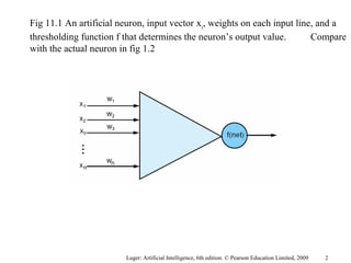
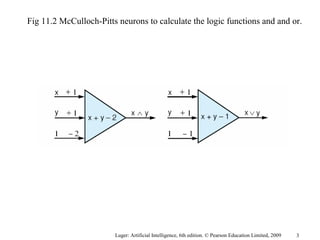
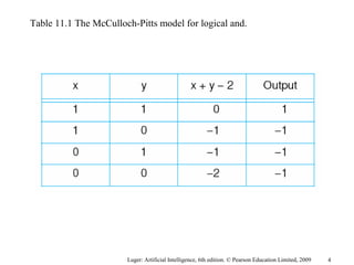
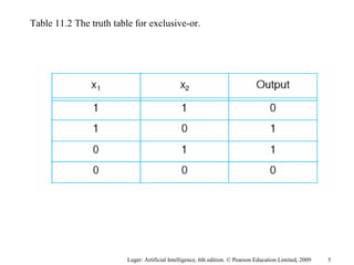
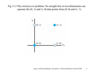
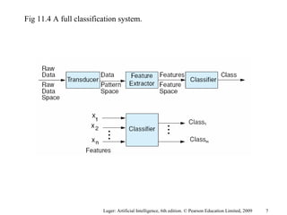
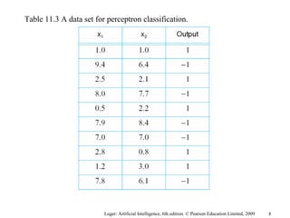
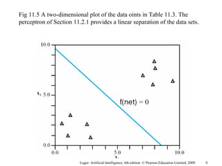
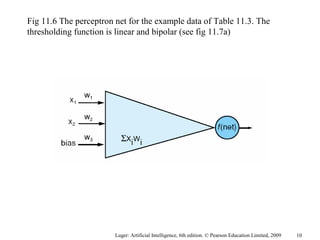
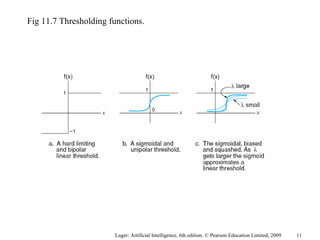
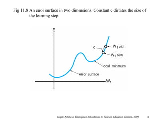
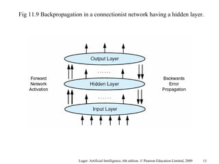
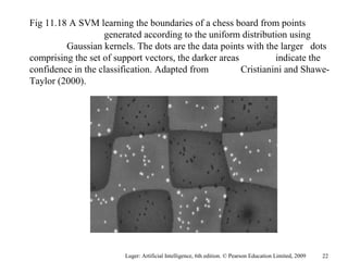
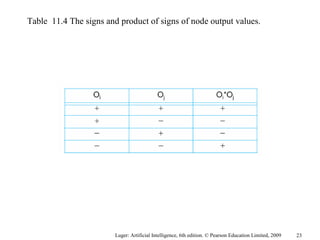
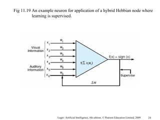
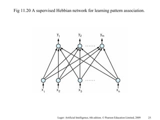
George F Luger
ARTIFICIAL INTELLIGENCE 6th edition
Structures and Strategies for Complex Problem Solving
Machine Learning: Connectionist
Luger: Artificial Intelligence, 6th edition. © Pearson Education Limited, 2009
11.0 Introduction
11.1 Foundations for Connectionist
Networks
11.2 Perceptron Learning
11.3 Backpropagation Learning.
11.4 Competitive Learning
11.5 Hebbian Coincidence Learning
11.6 Attractor Networks or “Memories”
11.7 Epilogue and References
11.8 Exercises
1

Fig 11.1 An artificial neuron, input vector xi
, weights on each input line, and a
thresholding function f that determines the neuron’s output value. Compare
with the actual neuron in fig 1.2
2

Fig 11.2 McCulloch-Pitts neurons to calculate the logic functions and and or.
3

Table 11.1 The McCulloch-Pitts model for logical and.
4

Table 11.2 The truth table for exclusive-or.
5

Fig 11.3 The exclusive-or problem. No straight line in two-dimensions can
separate the (0, 1) and (1, 0) data points from (0, 0) and (1, 1).
6

Fig 11.4 A full classification system.
7

Table 11.3 A data set for perceptron classification.
8

Fig 11.5 A two-dimensional plot of the data oints in Table 11.3. The
perceptron of Section 11.2.1 provides a linear separation of the data sets.
9

Fig 11.6 The perceptron net for the example data of Table 11.3. The
thresholding function is linear and bipolar (see fig 11.7a)
10
ΣX
iW
i

Fig 11.7 Thresholding functions.
11

Fig 11.8 An error surface in two dimensions. Constant c dictates the size of
the learning step.
12

Fig 11.9 Backpropagation in a connectionist network having a hidden layer.
13

Fig 11.10
14

Fig 11.11 The network topology of NETtalk.
15

Fig 11.12 A backpropagation net to solve the exclusive-or problem. The Wij
are the weights and H is the hidden node.
16

Fig 11.13 A layer of nodes for application of a winner-take-all algorithm. The
old input vectors support the winning node.
17

Fig 11.14 The use of a Kohonen layer, unsupervised, to generate a sequence
of prototypes to represent the classes of Table 11.3.
18

Fig 11.15 The architecture of the Kohonen based learning network for the
data of Table 11.3 and classification of Fig 11.4.
19

Fig 11.16 The “outstar” of node J, the “winner” in a winner-take-all network.
The Y vector supervises the response on the output layer in Grossberg
training. The “outstar” is bold with all weights, 1; all other weights are 0.
20

Fig 11.17 A counterpropagation network to recognize the classes in Table
11.3. We train the outstar weights of node A, wsa
and wda
.
21

Fig 11.18 A SVM learning the boundaries of a chess board from points
generated according to the uniform distribution using
Gaussian kernels. The dots are the data points with the larger dots
comprising the set of support vectors, the darker areas indicate the
confidence in the classification. Adapted from Cristianini and Shawe-
Taylor (2000).
22

Table 11.4 The signs and product of signs of node output values.
23

Fig 11.19 An example neuron for application of a hybrid Hebbian node where
learning is supervised.
24

Fig 11.20 A supervised Hebbian network for learning pattern association.
25

Fig 11.21 The linear association network. The vector Xi
is entered as input
and the associated vector Y is produced as output. yi
is a linear
combination of the x input. In training each yi
is supplied with its correct
output signals.
26

Fig 11.22 A linear associator network for the example in Section 11.5.4.
The weight matrix is calculated using the formula presented in the
previous section.
27

Fig 11.23 A BAM network for the examples of Section 11.6.2. Each node
may also be connected to itself.
28

Fig 11.24 An autoassociative network with an input vector Ii
. We assume
single links between nodes with unique indices, thus wij
= wij
and the weight matrix is symmetric.
29

Artificial Intelligence

More Related Content

What's hot

Viewers also liked

Similar to Artificial Intelligence

More from Muhammad Ahad

Recently uploaded

Artificial Intelligence