Download to read offline
![Problem Statement
A color image (mxn) is represented as three matrices of intensities
R,G,B ∈ Rmxn with entries in [0,1] representing the red, green, and
blue pixel intensities, respectively.
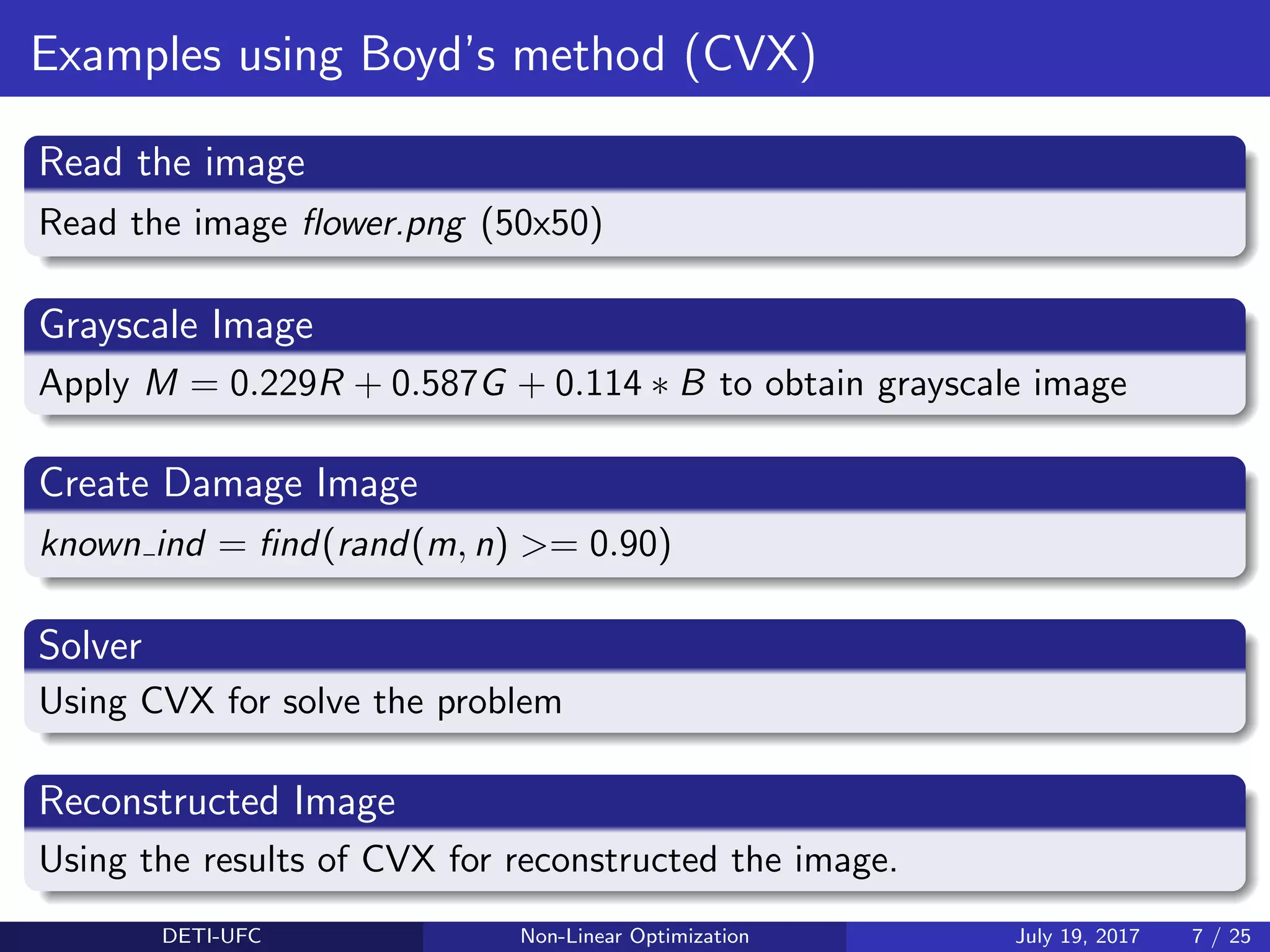
A color image is converted to a monochrome image, represented as
one matrix M ∈ Rmxn using
M = 0.299R + 0.587G + 0.114B (1)
DETI-UFC Non-Linear Optimization July 19, 2017 3 / 25](https://image.slidesharecdn.com/mainvf-170720151440/75/Colorization-with-total-variantion-regularization-3-2048.jpg)
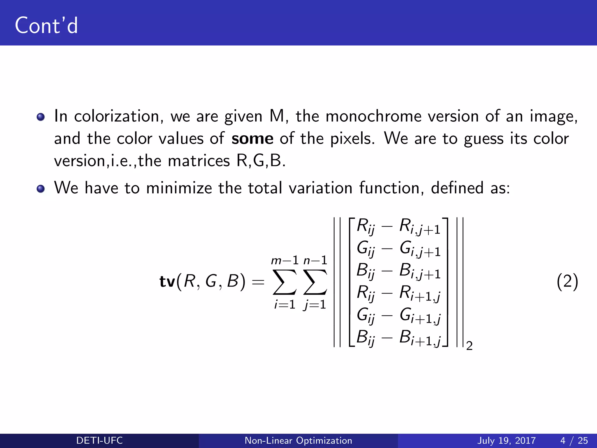
![Cont’d
Subject to consistency with the given monochrome image M, the
knows ranges of the entries of (R,G,B) (i.e.,∈ [0,1]), and the given
color entries.
Monochrome version of the image, M, along with vectors of known
color intensities is given to us.
The tv function, invoked as tv(R,G,B), gives the total variation.
Report your optimal objective value and if you have access to a color
printer, attach your reconstructed image.
If you don’t have access to a color printer, it’s OK to just give the
optimal objective value.
DETI-UFC Non-Linear Optimization July 19, 2017 5 / 25](https://image.slidesharecdn.com/mainvf-170720151440/75/Colorization-with-total-variantion-regularization-5-2048.jpg)
![Cont’d
Convex Problem
Every norms on Rn is convex!
minimize tv(R, G, B)
subject to:
R(knom ind) == R know
G(knom ind) == G know
B(knom ind) == B know
0.229R + 0.587G + 0.114B == M
R, G and B ∈ [0, 1] (3)
DETI-UFC Non-Linear Optimization July 19, 2017 6 / 25](https://image.slidesharecdn.com/mainvf-170720151440/75/Colorization-with-total-variantion-regularization-6-2048.jpg)
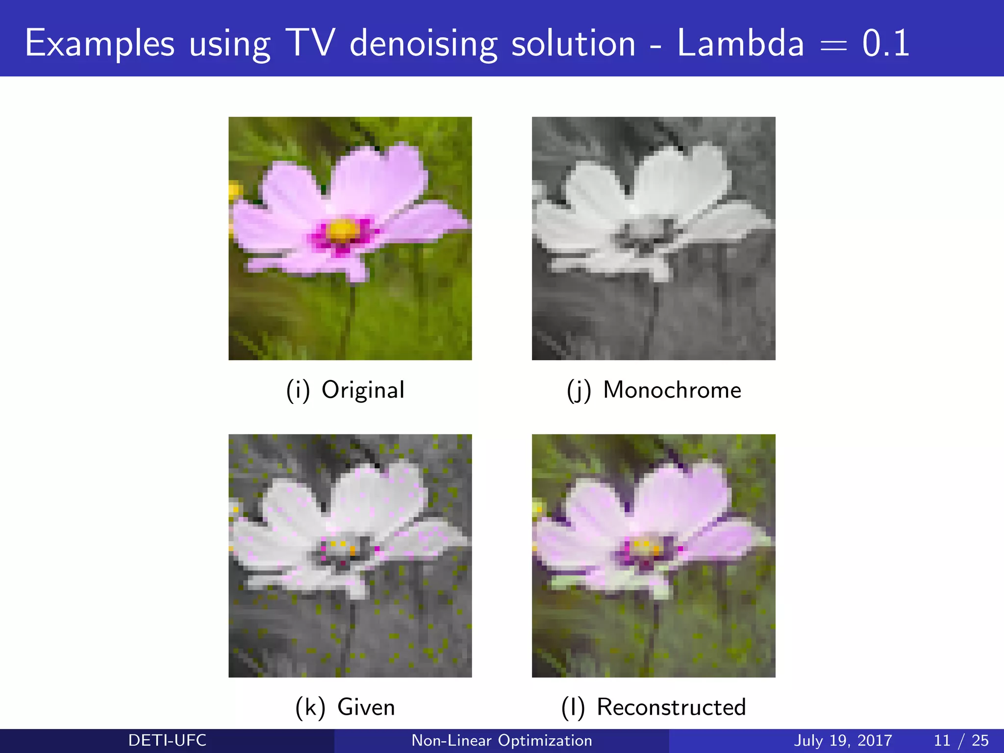
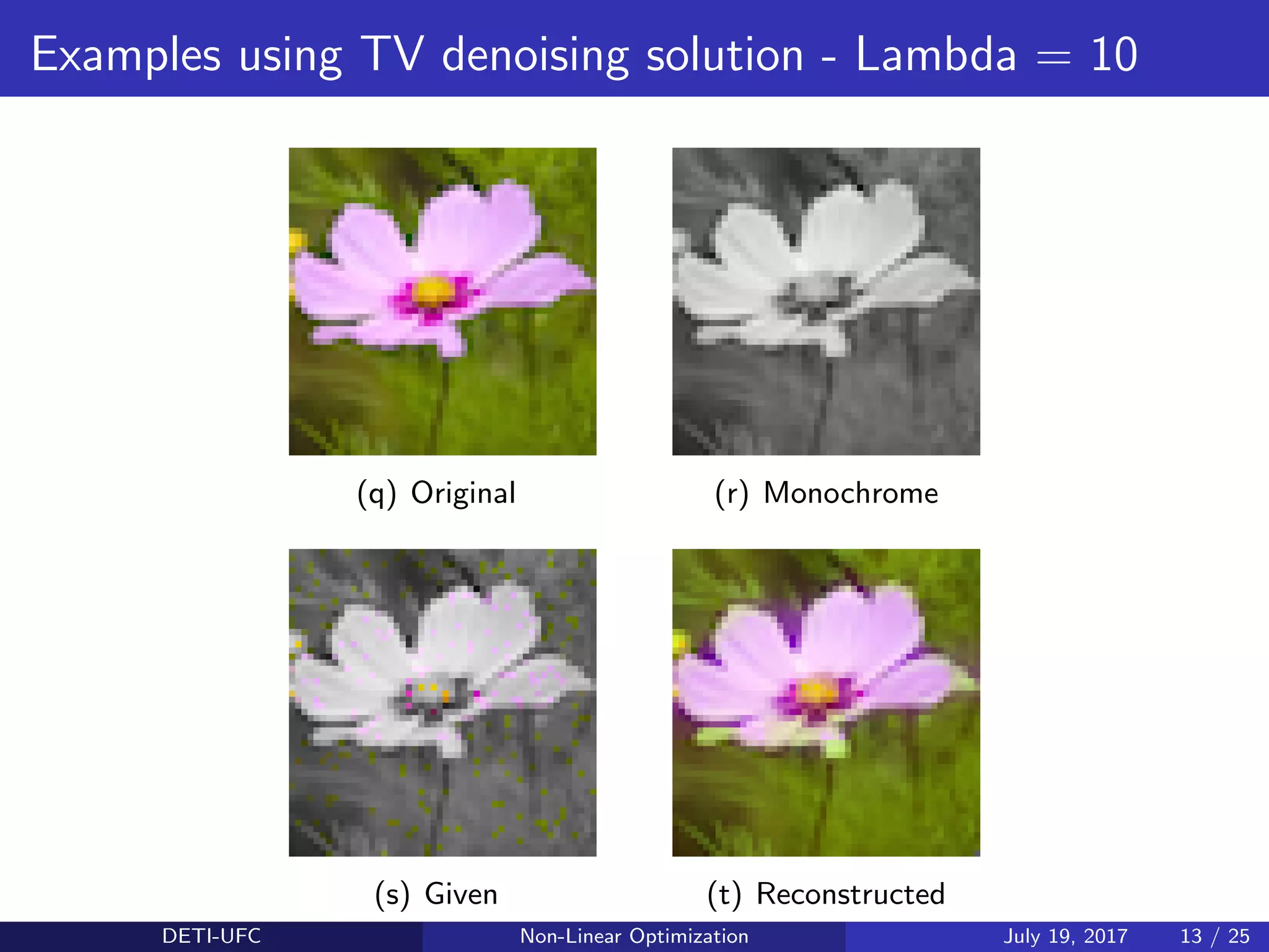
![TV denoising solution
minimize ||X − Y || + λ · tv(R, G, B)
subject to:
R(knom ind) == R know
G(knom ind) == G know
B(knom ind) == B know
0.229R + 0.587G + 0.114B == M
R, G and B ∈ [0, 1] (4)
Definition of variables
where X is the concatenation of R, G and B and Y is the monochromatic
image, in vector form.
λ is a positive scale factor.
DETI-UFC Non-Linear Optimization July 19, 2017 10 / 25](https://image.slidesharecdn.com/mainvf-170720151440/75/Colorization-with-total-variantion-regularization-10-2048.jpg)

![Metrics used for Comparison
Mean Square Error (MSE)
MSE =
1
MN
M
y=1
N
x=1
[I(x, y) − ˜I(x, y)]2
(7)
Peak Signal to Noise Ratio (PSNR)
PSNR = 20 ∗ log10
255
√
MSE
(8)
DETI-UFC Non-Linear Optimization July 19, 2017 20 / 25](https://image.slidesharecdn.com/mainvf-170720151440/75/Colorization-with-total-variantion-regularization-20-2048.jpg)
![References
1 S. Boyd and L. Vandenberghe. Convex Optimization. Cambridge
University Press, 2004.
2 S. Boyd, Jenny Hong el al. Convex Optimization in Julia. HPTCDL
November 16-21, 2014, New Orleans, Louisiana, USA
3 Karanveer Mohan, Madeleine Udell, David Zeng, Jenny Hong.
Convex.jl Documentation. Jun 24, 2017.
4 Nonlinear total variation based noise removal algorithms, Rudin, L. I.;
Osher, S.; Fatemi, E. (1992). Physica D 60: 259–268.
5 A generalized vector-valued total variation algorithm., Rodriguez
Paul, and Brendt Wohlberg. Image Processing (ICIP), 2009 16th
IEEE International Conference on. IEEE, 2009.
6 R´emi Flamary. Avaliable at:
http://remi.flamary.com/demos/proxtv.html [Acessed - 07/16]
7 LEVIN, A., LISCHINSKI, D., AND WEISS, Y. 2004. Colorization
using optimization. ACM Trans. Graph. 23, 3 (Aug.), 689–694.
DETI-UFC Non-Linear Optimization July 19, 2017 24 / 25](https://image.slidesharecdn.com/mainvf-170720151440/75/Colorization-with-total-variantion-regularization-24-2048.jpg)

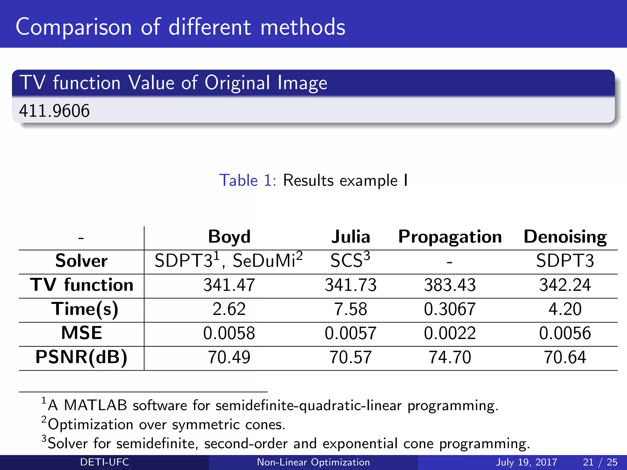
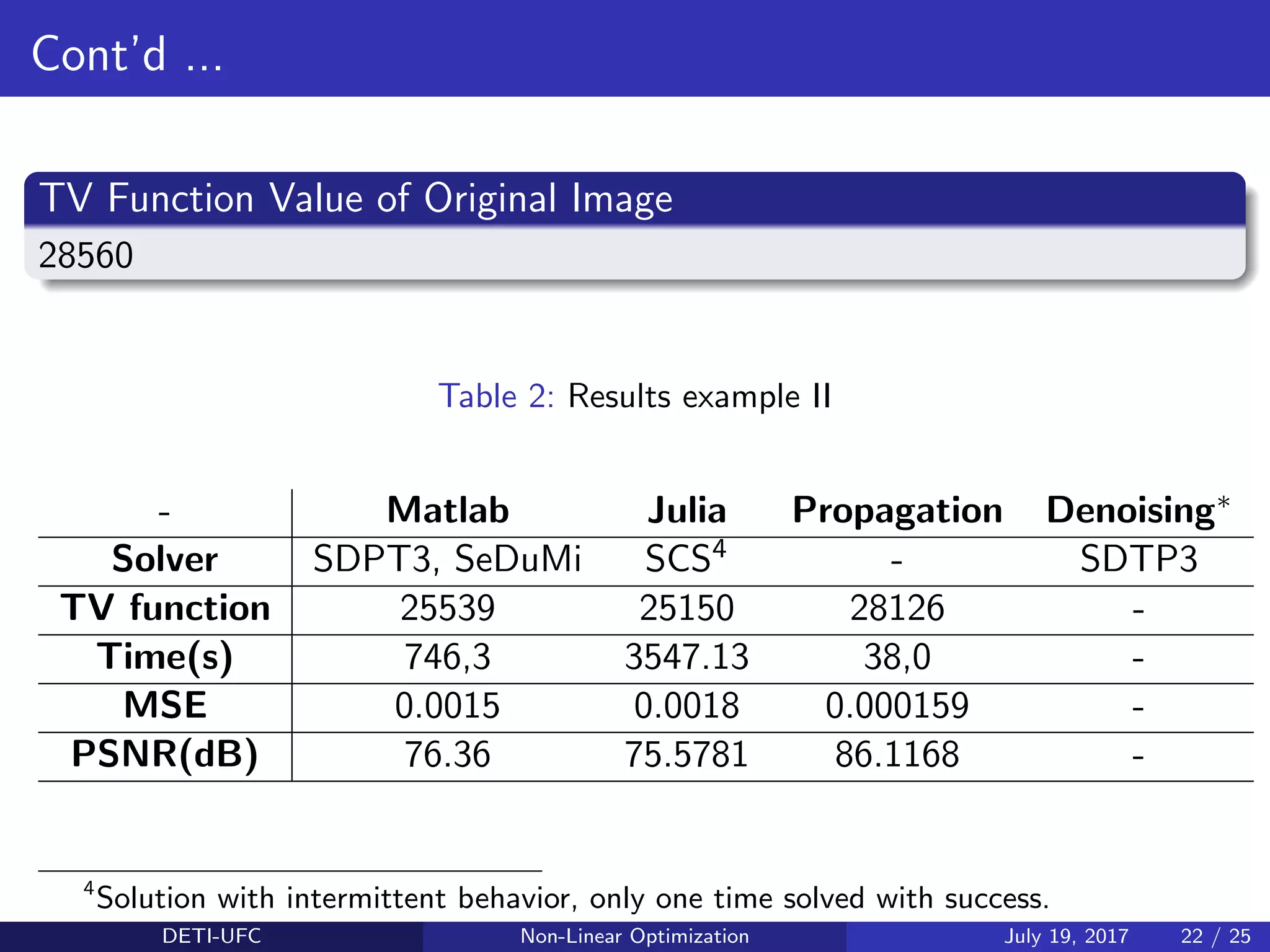
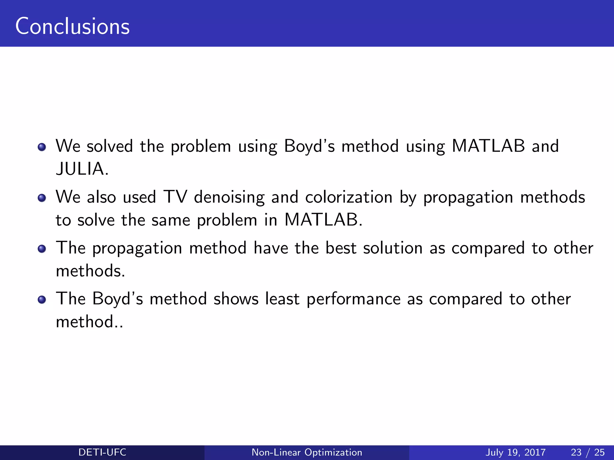
This document presents different methods for colorizing grayscale images, including total variation regularization, total variation denoising, and colorization by propagation. It outlines the problem statement, describes the various approaches, provides examples applying each method to images, and compares the results in terms of the total variation value, runtime, and image quality metrics. The propagation method achieved the best results with the lowest errors and highest PSNR values compared to other approaches like Boyd's method and total variation denoising.