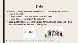
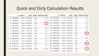
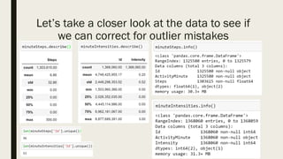
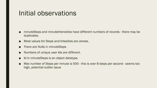
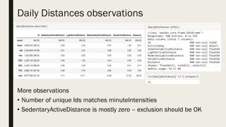
The document discusses the impact of dirty data on data analysis, particularly in spreadsheet formats like Excel, emphasizing the prevalence of issues such as duplicates, missing values, and outliers. It presents methods to handle and clean data, including single and multiple imputation techniques, and introduces the concept of 'tidy data' for effective organization. A case study using a Fitbit dataset illustrates the effects of data quality on analysis outcomes.

1. ANALYST’S
NIGHTMARE OR
LAUNDERING MASSIVE
SPREADSHEETS
An example of how analysis that overlooks data quality issues may go
completely wrong
By Feyzi Bagirov and Tanya Yarmola

2. Agenda
■ About us
■ Dirty Data types
■ Fit Bit dataset insights (pre-impute)
■ Fit Bit dataset insights (post-impute)
■ Q&A

3. About us
■ Vice President in
Model Governance
and Review at
JP Morgan
■ Faculty of Analytics at
Harrisburg University
of Science and
Technology
■ Data Science Advisor
at Metadata.io

4. According to Gartner, Excel is still the
most popular BI tool in the world
■ More and more powerful tools are available on the market
■ Spreadsheet however lives on:
– Excel is the most widely used analytics
tool in the world

6. Dirty Data
■ Significant quantities of data are stored and passed around in the spreadsheet
formats
■ Analysis is also frequently performed without leaving Excel.
■ This aggravates data quality issues:
– duplicates and nulls are overlooked
– copy-pastes and manual imputations create additional errors
– VLOOKUPS do not take duplicates into account
■ When the data happens to be not as clean as you hoped it to be, serious errors
occur and reproduce through the spreadsheet work cycle.

7. According to IDG, cleaning and organizing
data takes up to 60% of the data scientists’
time

8. Common types of dirty data
■ Missing data
– Missing Completely At Random (MCAR)
– Missing At Random (MAR)
– Missing Not At Random (MNAR)
■ Duplicates
■ Outliers
■ Multiple comma-separated (or not) values that are stored in one column (common
symptom)
■ Column headers are values, not variable names

9. Handling Dirty Data
■ You can handle dirty data on two levels:
– Database level/manual clean inside the database – not efficient, does not scale
well
– Application level – recommended way, whenever possible
Ø Identify the commonly occurring problems with your data and the tasks to fix them
Ø Once you identified most common tasks related to your data cleanup, create scripts, that you
are going to be run on every new dataset.
Ø Whenever you have new type of errors in the new dataset, add the code to fix them to your
scripts.

10. Concept of tidy data
■ “Tidy Data” by Hadley Wickham, “Journal of Statistical Software”, Aug 20141
■ Principles of tidy data:
– Observations as rows
– Variables of columns
– One type of observational unit per table (if table that suppose to contain
characteristics of people, contains information about their pets, there are more
observational units).
1 https://www.jstatsoft.org/article/view/v059i10/v59i10.pdf

11. Objectives
■ To provide a simple example that illustrates how data quality issues may visibly
affect results of an analysis
■ To estimate customer’s height based on average stride length and see whether
results belong to expected ranges

12. Tools

13. ■ https://zenodo.org/record/53894/files/mturkfitbit_export_4.12.16-5.12.16.zip
• A publicly available FitBit dataset1 that contains records on 33
customers with
• minute-by-minute records on steps and intensities
• daily distances travelled (FitBit estimate)
• Data quality issues were introduced for illustration purposes – this
also allows comparison with the original.
Data

14. Data

15. Quick an dirty height calculation

16. Quick and Dirty Calculation Results

17. Let’s take a closer look at the data to see if
we can correct for outlier mistakes

18. Initial observations
■ minuteSteps and minuteIntensities have different numbers of records - there may be
duplicates.
■ Most values for Steps and Intesities are zeroes.
■ There are Nulls in minuteSteps
■ Numbers of unique user Ids are different.
■ Id in minuteSteps is an object datatype.
■ Max number of Steps per minute is 500 - this is over 8 steps per second - seems too
high, potential outlier issue

19. Daily Distances observations
More observations
• Number of unique Ids matches minuteIntensities
• SedentaryActiveDistance is mostly zero – exclusion should be OK

20. Analysis with Data Checks
• Ids are mix of integers and strange strings
• Should convert all to integers to match other datasets

21. Analysis with Data Checks(cont’d)

22. Analysis with Data Checks(cont’d)

23. Nulls and outliers
• There are Nulls in minuteSteps
• Max number of Steps per minute is 500 - this is over 8 steps per
second - seems too high, potential outlier issue

24. Missing Values - Imputations
Imputation is used when the data analysis techniques is not content
robust. It can be done in several ways, but multiple imputations is
recommended and is a relatively standard method:
- Single imputation
- Multiple imputation

25. Single Imputations
■ Mean substitution - replacing missing value with the mean of that value for all other
cases. Does not change the sample mean for that variable, however, attenuates any
correlations involving the imputed variables, because there is no guaranteed
relationships between the imputed and measured variables)
■ Interpolation – a method of constructing new data points within the range of a
discrete set of known data points.

26. ■ Partial deletion (Listwise deletion/casewise)- the most common means of dealing
with missing data is listwise deletion (complete case), which is when all cases with
missing values are deleted. If the data are MCAR, this will not add any bias, but it
will decrease the power of the analysis (smaller sample size).
■ Pairwise deletion – deleting a case when it is missing a variable required for a
particular analysis, but including that case in analysis for which all required
variables are present. The main advantage of this method is that it is
straightforward and easy to implement.
Single Imputations (cont’d)

27. ■ Hot-deck – a missing value is imputed from a randomly selected similar record.
■ Cold deck – selects donors from another dataset. Due to the advances in
computation power, more sophisticated methods have superseded the original
random and sorted hot deck imputation techniques
■ Regression imputation - Available information for complete and incomplete cases is
used to predict whether a value on a specific variable is missing or not. Fitted values
from the regression model are then used to impute the missing values. It has the
opposite problem of mean imputation – imputed data do not have an error term
included in their estimation, thus the estimates fit perfectly along the regression line
without any residual variance, causing relationships to be over identified and
suggest greater precision in the imputed values, supplying no uncertainty about that
value.
Single Imputations (cont’d)

28. Multiple Imputations
■ Multiple Imputation developed to deal with the problem of increased noise due to
imputation by Rubin (1987). There are multiple methods of multiple imputation
■ The primary method is Multiple Imputation by Chained Equations (MICE) should be
implemented only when the missing data follow the missing at random mechanism

29. Multiple Imputations (cont’d)
■ Advantages of Multiple Imputation:
– An advantage over single imputation is that MI is flexible and can be used in cases,
where the data is MCAR, MAR, and even when the data is MNAR.
– By imputing multiple times, multiple imputation certainly accounts for the
uncertainty and range of values that the true value could have taken.
– Not difficult to implement
■ Disadvantages of Multiple Imputation:
– Can be computationally expensive and not quite worth it.

30. Steps distributions per intensity
Single imputations - Impute nulls and outliers
using different methods:
1. mean value
2. interpolate between existing values
3. draw from the distribution of existing
values (per customer)

31. Single imputation - Impute using mean

32. Single imputation - impute using
interpolation

33. Impute using transform with random
choice (hot-deck)

34. Calculate height function

35. Calculate height for different imputation
versions and compare results

37. Q&A

38. Thanks!
Feyzi Bagirov, feyzi.bagirov@metadata.io, @FeyziBagirov
Tanya Yarmola, tanya.yarmola@jpmorgan.com, @TanyaYarmola