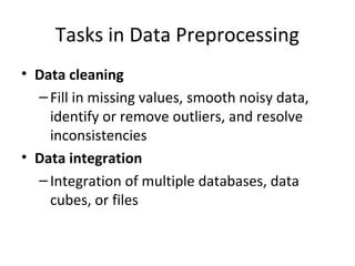
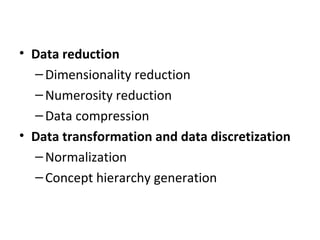
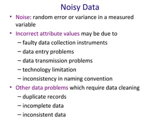
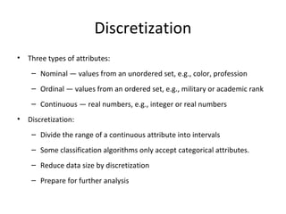
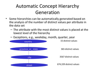
Data Preprocessing
M.Ganeshkumar
Why Preprocess the Data?
• Data in the real world is dirty

– incomplete: lacking attribute values, lacking certain
attributes of interest, or containing only aggregate
data
• e.g., occupation=“ ”

– noisy: containing errors or outliers
• e.g., Salary=“-10”

– inconsistent: containing discrepancies in codes or
names
• e.g., Age=“42” Birthday=“03/07/1997”
• e.g., Was rating “1,2,3”, now rating “A, B, C”
• e.g., discrepancy between duplicate records
Tasks in Data Preprocessing
• Data cleaning
– Fill in missing values, smooth noisy data,
identify or remove outliers, and resolve
inconsistencies
• Data integration
– Integration of multiple databases, data
cubes, or files
• Data reduction
– Dimensionality reduction
– Numerosity reduction
– Data compression
• Data transformation and data discretization
– Normalization
– Concept hierarchy generation
Data Cleaning
• Data in the Real World Is Dirty: Lots of potentially incorrect
data, e.g., instrument faulty, human or computer error,
transmission error
– incomplete: lacking attribute values, lacking certain
attributes of interest, or containing only aggregate data
• e.g., Occupation = “ ” (missing data)
– noisy: containing noise, errors, or outliers
• e.g., Salary = “−10” (an error)
– inconsistent: containing discrepancies in codes or
names, e.g.,
• Age = “42”, Birthday = “03/07/2010”
• Was rating “1, 2, 3”, now rating “A, B, C”
• discrepancy between duplicate records
– Intentional (e.g., disguised missing data)
• Jan. 1 as everyone’s birthday?
Incomplete (Missing) Data
• Data is not always available
– E.g., many tuples have no recorded value for several
attributes, such as customer income in sales data
• Missing data may be due to
– equipment malfunction
– inconsistent with other recorded data and thus deleted
– data not entered due to misunderstanding
– certain data may not be considered important at the time
of entry
– not register history or changes of the data
• Missing data may need to be inferred
How to Handle Missing Data
• Ignore the tuple: usually done when class label is missing
(when doing classification)—not effective when the % of
missing values per attribute varies considerably
• Fill in the missing value manually: tedious + infeasible?
• Fill in it automatically with
– a global constant : e.g., “unknown”, a new class?!
– the attribute mean
– the attribute mean for all samples belonging to the same
class: smarter
– the most probable value: inference-based such as
Bayesian formula or decision tree
Noisy Data
• Noise: random error or variance in a measured
variable
• Incorrect attribute values may be due to
– faulty data collection instruments
– data entry problems
– data transmission problems
– technology limitation
– inconsistency in naming convention
• Other data problems which require data cleaning
– duplicate records
– incomplete data
– inconsistent data
Handle Noisy Data

• Binning
– first sort data and partition into (equal-frequency)
bins
– then one can smooth by bin means, smooth by bin
median, smooth by bin boundaries, etc.
• Regression
– smooth by fitting the data into regression
functions
• Clustering
– detect and remove outliers
• Combined computer and human inspection
– detect suspicious values and check by human
(e.g., deal with possible outliers)
Data Cleaning

• Importance
– “Data cleaning is one of the three biggest problems in data
warehousing”—Ralph Kimball
– “Data cleaning is the number one problem in data
warehousing”—DCI survey
• Data cleaning tasks
– Fill in missing values
– Identify outliers and smooth out noisy data
– Correct inconsistent data
– Resolve redundancy caused by data integration
Missing Data
•

Data is not always available
– E.g., many tuples have no recorded value for several attributes, such
as customer income in sales data

•

Missing data may be due to
– equipment malfunction
– inconsistent with other recorded data and thus deleted
– data not entered due to misunderstanding
– certain data may not be considered important at the time of entry
– not register history or changes of the data

•

Missing data may need to be inferred.
Handle Missing Data
•

Ignore the tuple: usually done when class label is missing (assuming the tasks
in classification—not effective when the percentage of missing values per
attribute varies considerably.

•

Fill in the missing value manually: tedious + infeasible?

•

Fill in it automatically with
– a global constant : e.g., “unknown”, a new class?!
– the attribute mean
– the attribute mean for all samples belonging to the same class: smarter
– the most probable value: inference-based such as Bayesian formula or
decision tree
Binning Methods for Data
Smoothing
 Sorted data for price (in dollars): 4, 8, 9, 15, 21, 21, 24, 25, 26, 28, 29, 34
* Partition into equal-frequency (equi-depth) bins:
- Bin 1: 4, 8, 9, 15
- Bin 2: 21, 21, 24, 25
- Bin 3: 26, 28, 29, 34
* Smoothing by bin means:
- Bin 1: 9, 9, 9, 9
- Bin 2: 23, 23, 23, 23
- Bin 3: 29, 29, 29, 29
* Smoothing by bin boundaries:
- Bin 1: 4, 4, 4, 15
- Bin 2: 21, 21, 25, 25
- Bin 3: 26, 26, 26, 34
February 19, 2008

14
Regression
y

Y1
y=x+1

Y1’

X1

February 19, 2008

x

15
Cluster Analysis

February 19, 2008

16
Data Integration
•

Data integration:
– Combines data from multiple sources into a coherent store

•

Schema integration: e.g., A.cust-id ≡ B.cust-#
– Integrate metadata from different sources

•

Entity identification problem:
– Identify real world entities from multiple data sources, e.g., Bill Clinton =
William Clinton

•

Detecting and resolving data value conflicts
– For the same real world entity, attribute values from different sources are
different
– Possible reasons: different representations, different scales, e.g., metric
vs. British units
Handling Redundancy in Data
Integration
• Redundant data occur often when integration of multiple databases
– Object identification: The same attribute or object may have
different names in different databases
– Derivable data: One attribute may be a “derived” attribute in
another table, e.g., annual revenue
• Redundant attributes may be able to be detected by correlation
analysis and covariance analysis
• Careful integration of the data from multiple sources may help
reduce/avoid redundancies and inconsistencies and improve mining
speed and quality
Correlation Analysis (Nominal Data)
• Χ2 (chi-square) test

(Observed − Expected ) 2
2
χ =∑
Expected

• The larger the Χ2 value, the more likely the variables are
related
• The cells that contribute the most to the Χ2 value are those
whose actual count is very different from the expected count
• Correlation does not imply causality
– # of hospitals and # of car-theft in a city are correlated
– Both are causally linked to the third variable: population
Correlation Analysis (Numeric Data)
• Correlation coefficient (also called Pearson’s product moment
coefficient)

where n is the number of tuples,
and are the
respective means of A and B, σA and σB are the respective
standard deviation of A and B, and Σ(aibi) is the sum of the
AB cross-product.
• If rA,B > 0, A and B are positively correlated (A’s values increase
as B’s). The higher, the stronger correlation.
• rA,B = 0: independent; rAB < 0: negatively correlated
Visually Evaluating Correlation
Correlation (viewed as linear
relationship)
•Correlation measures the linear relationship between
objects
•To compute correlation, we standardize data objects,
A and B, and then take their dot product

a 'k = (ak − mean( A)) / std ( A)
b'k = (bk − mean( B )) / std ( B)
correlation( A, B) = A'• B '
Data Reduction 1: Dimensionality
Reduction
•

•

•

Curse of dimensionality
– When dimensionality increases, data becomes increasingly sparse
– Density and distance between points, which is critical to clustering, outlier
analysis, becomes less meaningful
– The possible combinations of subspaces will grow exponentially
Dimensionality reduction
– Avoid the curse of dimensionality
– Help eliminate irrelevant features and reduce noise
– Reduce time and space required in data mining
– Allow easier visualization
Dimensionality reduction techniques
– Wavelet transforms
– Principal Component Analysis
– Supervised and nonlinear techniques (e.g., feature selection)
Data Reduction Strategies
•
•
•

Data reduction: Obtain a reduced representation of the data set that is
much smaller in volume but yet produces the same (or almost the same)
analytical results
Why data reduction? — A database/data warehouse may store terabytes
of data. Complex data analysis may take a very long time to run on the
complete data set.
Data reduction strategies
– Dimensionality reduction, e.g., remove unimportant attributes
• Wavelet transforms
• Principal Components Analysis (PCA)
• Feature subset selection, feature creation
– Numerosity reduction (some simply call it: Data Reduction)
• Regression and Log-Linear Models
• Histograms, clustering, sampling
• Data cube aggregation
– Data compression
Mapping Data to a New Space



Fourier transform
Wavelet transform

Two Sine Waves

Two Sine Waves + Noise

Frequency
Data Transformation
• Smoothing: remove noise from data
• Aggregation: summarization, data cube construction
• Generalization: concept hierarchy climbing
• Normalization: scaled to fall within a small, specified range
– min-max normalization
– z-score normalization
– normalization by decimal scaling
• Attribute/feature construction
– New attributes constructed from the given ones
Data Reduction Strategies
•

•

•

Why data reduction?
– A database/data warehouse may store terabytes of data
– Complex data analysis/mining may take a very long time to run on the
complete data set
Data reduction
– Obtain a reduced representation of the data set that is much smaller in
volume but yet produce the same (or almost the same) analytical results
Data reduction strategies
– Data cube aggregation:
– Dimensionality reduction — e.g., remove unimportant attributes
– Data Compression
– Numerosity reduction — e.g., fit data into models
– Discretization and concept hierarchy generation
Attribute Subset Selection
• Feature selection (i.e., attribute subset selection):
– Select a minimum set of features such that the probability
distribution of different classes given the values for those
features is as close as possible to the original distribution
given the values of all features
– reduce # of patterns in the patterns, easier to understand
• Heuristic methods (due to exponential # of choices):
– Step-wise forward selection
– Step-wise backward elimination
– Combining forward selection and backward elimination
– Decision-tree induction
Example of Decision Tree Induction
Initial attribute set:
{A1, A2, A3, A4, A5, A6}

A4 ?

A6?

A1?

Class 1
>

Class 2

Class 1

Reduced attribute set: {A1, A4, A6}

Class 2
Heuristic Feature Selection Methods
• There are 2d possible sub-features of d features
• Several heuristic feature selection methods:
– Best single features under the feature independence
assumption: choose by significance tests
– Best step-wise feature selection:
• The best single-feature is picked first
• Then next best feature condition to the first, ...
– Step-wise feature elimination:
• Repeatedly eliminate the worst feature
– Best combined feature selection and elimination
– Optimal branch and bound:
• Use feature elimination and backtracking
Numerosity Reduction
• Reduce data volume by choosing alternative, smaller forms of
data representation
• Parametric methods
– Assume the data fits some model, estimate model
parameters, store only the parameters, and discard the
data (except possible outliers)
– Example: Log-linear models—obtain value at a point in mD space as the product on appropriate marginal subspaces
• Non-parametric methods
– Do not assume models
– Major families: histograms, clustering, sampling
Data Reduction Method (1):
Regression and Log-Linear Models
• Linear regression: Data are modeled to fit a straight line
– Often uses the least-square method to fit the line
• Multiple regression: allows a response variable Y to be
modeled as a linear function of multidimensional feature
vector
• Log-linear model: approximates discrete multidimensional
probability distributions
Data Reduction Method (2):
Histograms
•

Divide data into buckets and store
average (sum) for each bucket

•

Partitioning rules:

40
35

– Equal-width: equal bucket range

30

– Equal-frequency (or equal-depth)

25
15
10
5

100000

90000

80000

70000

60000

50000

40000

30000

0
20000

– MaxDiff: set bucket boundary
between each pair for pairs have
the β–1 largest differences

20

10000

– V-optimal: with the least
histogram variance (weighted
sum of the original values that
each bucket represents)
Data Reduction Method (3): Clustering
• Partition data set into clusters based on similarity, and
store cluster representation (e.g., centroid and diameter)
only
• Can be very effective if data is clustered but not if data is
“smeared”
• Can have hierarchical clustering and be stored in multidimensional index tree structures
• There are many choices of clustering definitions and
clustering algorithms
• Cluster analysis will be studied in depth in Chapter 7
Data Reduction Method (4): Sampling
• Sampling: obtaining a small sample s to represent the whole
data set N
• Allow a mining algorithm to run in complexity that is
potentially sub-linear to the size of the data
• Choose a representative subset of the data
– Simple random sampling may have very poor performance
in the presence of skew
• Develop adaptive sampling methods
– Stratified sampling:
• Approximate the percentage of each class (or
subpopulation of interest) in the overall database
• Used in conjunction with skewed data
• Note: Sampling may not reduce database I/Os (page at a time)
Sampling: with or without
Replacement

R
SWO andom
SR
r
mple without
(si
le
samp ement)
c
repla

SRSW
R

Raw Data
Sampling: Cluster or Stratified Sampling

Raw Data

Cluster/Stratified Sample
Discretization
•

Three types of attributes:
– Nominal — values from an unordered set, e.g., color, profession
– Ordinal — values from an ordered set, e.g., military or academic rank
– Continuous — real numbers, e.g., integer or real numbers

•

Discretization:
– Divide the range of a continuous attribute into intervals
– Some classification algorithms only accept categorical attributes.
– Reduce data size by discretization
– Prepare for further analysis
Discretization and Concept Hierarchy
•

Discretization
– Reduce the number of values for a given continuous attribute by
dividing the range of the attribute into intervals
– Interval labels can then be used to replace actual data values
– Supervised vs. unsupervised
– Split (top-down) vs. merge (bottom-up)
– Discretization can be performed recursively on an attribute

•

Concept hierarchy formation
– Recursively reduce the data by collecting and replacing low level
concepts (such as numeric values for age) by higher level concepts
(such as young, middle-aged, or senior)
Discretization and Concept Hierarchy
Generation for Numeric Data
•

Typical methods: All the methods can be applied recursively
– Binning (covered above)
• Top-down split, unsupervised,
– Histogram analysis (covered above)
• Top-down split, unsupervised
– Clustering analysis (covered above)
• Either top-down split or bottom-up merge, unsupervised
– Entropy-based discretization: supervised, top-down split
– Interval merging by χ2 Analysis: unsupervised, bottom-up merge
– Segmentation by natural partitioning: top-down split, unsupervised
Segmentation by Natural Partitioning
•

A simply 3-4-5 rule can be used to segment numeric data
into relatively uniform, “natural” intervals.
– If an interval covers 3, 6, 7 or 9 distinct values at the
most significant digit, partition the range into 3 equiwidth intervals
– If it covers 2, 4, or 8 distinct values at the most significant
digit, partition the range into 4 intervals
– If it covers 1, 5, or 10 distinct values at the most
significant digit, partition the range into 5 intervals
Example of 3-4-5 Rule
count

-$351

Step 1:

-$159

Min
Step 2:

profit

Low (i.e, 5%-tile)

msd=1,000

Low=-$1,000

High(i.e, 95%-0 tile)

$4,700
Max

High=$2,000
(-$1,000 - $2,000)

Step 3:
(-$1,000 - 0)

(0 -$ 1,000)

($1,000 - $2,000)

(-$400 -$5,000)

Step 4:

(-$400 - 0)
(-$400 -$300)
(-$300 -$200)
(-$200 -$100)
(-$100 0)

$1,838

February 19, 2008

($1,000 - $2, 000)

(0 - $1,000)
(0 $200)

($1,000 $1,200)

($200 $400)

($600 $800)

($2,000 $3,000)

($1,200 $1,400)

($3,000 $4,000)

($1,400 $1,600)

($400 $600)
($800 $1,000)

($1,600 $1,800)

($2,000 - $5, 000)

($1,800 $2,000)

($4,000 $5,000)

42
Concept Hierarchy Generation for
Categorical Data
• Specification of a partial/total ordering of attributes explicitly at the
schema level by users or experts
– street < city < state < country
• Specification of a hierarchy for a set of values by explicit data
grouping
– {Urbana, Champaign, Chicago} < Illinois
• Specification of only a partial set of attributes
– E.g., only street < city, not others
• Automatic generation of hierarchies (or attribute levels) by the
analysis of the number of distinct values
– E.g., for a set of attributes: {street, city, state, country}
Automatic Concept Hierarchy
Generation
• Some hierarchies can be automatically generated based on
the analysis of the number of distinct values per attribute in
the data set
– The attribute with the most distinct values is placed at the
lowest level of the hierarchy
– Exceptions, e.g., weekday, month, quarter, year
country
province_or_ state
city
street

15 distinct values
365 distinct values
3567 distinct values
674,339 distinct values

Data preprocessing

  • 1.
  • 2.
    Why Preprocess theData? • Data in the real world is dirty – incomplete: lacking attribute values, lacking certain attributes of interest, or containing only aggregate data • e.g., occupation=“ ” – noisy: containing errors or outliers • e.g., Salary=“-10” – inconsistent: containing discrepancies in codes or names • e.g., Age=“42” Birthday=“03/07/1997” • e.g., Was rating “1,2,3”, now rating “A, B, C” • e.g., discrepancy between duplicate records
  • 3.
    Tasks in DataPreprocessing • Data cleaning – Fill in missing values, smooth noisy data, identify or remove outliers, and resolve inconsistencies • Data integration – Integration of multiple databases, data cubes, or files
  • 4.
    • Data reduction –Dimensionality reduction – Numerosity reduction – Data compression • Data transformation and data discretization – Normalization – Concept hierarchy generation
  • 5.
    Data Cleaning • Datain the Real World Is Dirty: Lots of potentially incorrect data, e.g., instrument faulty, human or computer error, transmission error – incomplete: lacking attribute values, lacking certain attributes of interest, or containing only aggregate data • e.g., Occupation = “ ” (missing data) – noisy: containing noise, errors, or outliers • e.g., Salary = “−10” (an error)
  • 6.
    – inconsistent: containingdiscrepancies in codes or names, e.g., • Age = “42”, Birthday = “03/07/2010” • Was rating “1, 2, 3”, now rating “A, B, C” • discrepancy between duplicate records – Intentional (e.g., disguised missing data) • Jan. 1 as everyone’s birthday?
  • 7.
    Incomplete (Missing) Data •Data is not always available – E.g., many tuples have no recorded value for several attributes, such as customer income in sales data • Missing data may be due to – equipment malfunction – inconsistent with other recorded data and thus deleted – data not entered due to misunderstanding – certain data may not be considered important at the time of entry – not register history or changes of the data • Missing data may need to be inferred
  • 8.
    How to HandleMissing Data • Ignore the tuple: usually done when class label is missing (when doing classification)—not effective when the % of missing values per attribute varies considerably • Fill in the missing value manually: tedious + infeasible? • Fill in it automatically with – a global constant : e.g., “unknown”, a new class?! – the attribute mean – the attribute mean for all samples belonging to the same class: smarter – the most probable value: inference-based such as Bayesian formula or decision tree
  • 9.
    Noisy Data • Noise:random error or variance in a measured variable • Incorrect attribute values may be due to – faulty data collection instruments – data entry problems – data transmission problems – technology limitation – inconsistency in naming convention • Other data problems which require data cleaning – duplicate records – incomplete data – inconsistent data
  • 10.
    Handle Noisy Data •Binning – first sort data and partition into (equal-frequency) bins – then one can smooth by bin means, smooth by bin median, smooth by bin boundaries, etc. • Regression – smooth by fitting the data into regression functions • Clustering – detect and remove outliers • Combined computer and human inspection – detect suspicious values and check by human (e.g., deal with possible outliers)
  • 11.
    Data Cleaning • Importance –“Data cleaning is one of the three biggest problems in data warehousing”—Ralph Kimball – “Data cleaning is the number one problem in data warehousing”—DCI survey • Data cleaning tasks – Fill in missing values – Identify outliers and smooth out noisy data – Correct inconsistent data – Resolve redundancy caused by data integration
  • 12.
    Missing Data • Data isnot always available – E.g., many tuples have no recorded value for several attributes, such as customer income in sales data • Missing data may be due to – equipment malfunction – inconsistent with other recorded data and thus deleted – data not entered due to misunderstanding – certain data may not be considered important at the time of entry – not register history or changes of the data • Missing data may need to be inferred.
  • 13.
    Handle Missing Data • Ignorethe tuple: usually done when class label is missing (assuming the tasks in classification—not effective when the percentage of missing values per attribute varies considerably. • Fill in the missing value manually: tedious + infeasible? • Fill in it automatically with – a global constant : e.g., “unknown”, a new class?! – the attribute mean – the attribute mean for all samples belonging to the same class: smarter – the most probable value: inference-based such as Bayesian formula or decision tree
  • 14.
    Binning Methods forData Smoothing  Sorted data for price (in dollars): 4, 8, 9, 15, 21, 21, 24, 25, 26, 28, 29, 34 * Partition into equal-frequency (equi-depth) bins: - Bin 1: 4, 8, 9, 15 - Bin 2: 21, 21, 24, 25 - Bin 3: 26, 28, 29, 34 * Smoothing by bin means: - Bin 1: 9, 9, 9, 9 - Bin 2: 23, 23, 23, 23 - Bin 3: 29, 29, 29, 29 * Smoothing by bin boundaries: - Bin 1: 4, 4, 4, 15 - Bin 2: 21, 21, 25, 25 - Bin 3: 26, 26, 26, 34 February 19, 2008 14
  • 15.
  • 16.
  • 17.
    Data Integration • Data integration: –Combines data from multiple sources into a coherent store • Schema integration: e.g., A.cust-id ≡ B.cust-# – Integrate metadata from different sources • Entity identification problem: – Identify real world entities from multiple data sources, e.g., Bill Clinton = William Clinton • Detecting and resolving data value conflicts – For the same real world entity, attribute values from different sources are different – Possible reasons: different representations, different scales, e.g., metric vs. British units
  • 18.
    Handling Redundancy inData Integration • Redundant data occur often when integration of multiple databases – Object identification: The same attribute or object may have different names in different databases – Derivable data: One attribute may be a “derived” attribute in another table, e.g., annual revenue • Redundant attributes may be able to be detected by correlation analysis and covariance analysis • Careful integration of the data from multiple sources may help reduce/avoid redundancies and inconsistencies and improve mining speed and quality
  • 19.
    Correlation Analysis (NominalData) • Χ2 (chi-square) test (Observed − Expected ) 2 2 χ =∑ Expected • The larger the Χ2 value, the more likely the variables are related • The cells that contribute the most to the Χ2 value are those whose actual count is very different from the expected count • Correlation does not imply causality – # of hospitals and # of car-theft in a city are correlated – Both are causally linked to the third variable: population
  • 20.
    Correlation Analysis (NumericData) • Correlation coefficient (also called Pearson’s product moment coefficient) where n is the number of tuples, and are the respective means of A and B, σA and σB are the respective standard deviation of A and B, and Σ(aibi) is the sum of the AB cross-product. • If rA,B > 0, A and B are positively correlated (A’s values increase as B’s). The higher, the stronger correlation. • rA,B = 0: independent; rAB < 0: negatively correlated
  • 21.
  • 22.
    Correlation (viewed aslinear relationship) •Correlation measures the linear relationship between objects •To compute correlation, we standardize data objects, A and B, and then take their dot product a 'k = (ak − mean( A)) / std ( A) b'k = (bk − mean( B )) / std ( B) b'k = (bk − mean( B )) / std ( B) correlation( A, B) = A'• B ' correlation( A, B) = A'• B '
  • 23.
    Data Reduction 1:Dimensionality Reduction • • • Curse of dimensionality – When dimensionality increases, data becomes increasingly sparse – Density and distance between points, which is critical to clustering, outlier analysis, becomes less meaningful – The possible combinations of subspaces will grow exponentially Dimensionality reduction – Avoid the curse of dimensionality – Help eliminate irrelevant features and reduce noise – Reduce time and space required in data mining – Allow easier visualization Dimensionality reduction techniques – Wavelet transforms – Principal Component Analysis – Supervised and nonlinear techniques (e.g., feature selection)
  • 24.
    Data Reduction Strategies • • • Datareduction: Obtain a reduced representation of the data set that is much smaller in volume but yet produces the same (or almost the same) analytical results Why data reduction? — A database/data warehouse may store terabytes of data. Complex data analysis may take a very long time to run on the complete data set. Data reduction strategies – Dimensionality reduction, e.g., remove unimportant attributes • Wavelet transforms • Principal Components Analysis (PCA) • Feature subset selection, feature creation – Numerosity reduction (some simply call it: Data Reduction) • Regression and Log-Linear Models • Histograms, clustering, sampling • Data cube aggregation – Data compression
  • 25.
    Mapping Data toa New Space   Fourier transform Wavelet transform Two Sine Waves Two Sine Waves + Noise Frequency
  • 26.
    Data Transformation • Smoothing:remove noise from data • Aggregation: summarization, data cube construction • Generalization: concept hierarchy climbing • Normalization: scaled to fall within a small, specified range – min-max normalization – z-score normalization – normalization by decimal scaling • Attribute/feature construction – New attributes constructed from the given ones
  • 27.
    Data Reduction Strategies • • • Whydata reduction? – A database/data warehouse may store terabytes of data – Complex data analysis/mining may take a very long time to run on the complete data set Data reduction – Obtain a reduced representation of the data set that is much smaller in volume but yet produce the same (or almost the same) analytical results Data reduction strategies – Data cube aggregation: – Dimensionality reduction — e.g., remove unimportant attributes – Data Compression – Numerosity reduction — e.g., fit data into models – Discretization and concept hierarchy generation
  • 28.
    Attribute Subset Selection •Feature selection (i.e., attribute subset selection): – Select a minimum set of features such that the probability distribution of different classes given the values for those features is as close as possible to the original distribution given the values of all features – reduce # of patterns in the patterns, easier to understand • Heuristic methods (due to exponential # of choices): – Step-wise forward selection – Step-wise backward elimination – Combining forward selection and backward elimination – Decision-tree induction
  • 29.
    Example of DecisionTree Induction Initial attribute set: {A1, A2, A3, A4, A5, A6} A4 ? A6? A1? Class 1 > Class 2 Class 1 Reduced attribute set: {A1, A4, A6} Class 2
  • 30.
    Heuristic Feature SelectionMethods • There are 2d possible sub-features of d features • Several heuristic feature selection methods: – Best single features under the feature independence assumption: choose by significance tests – Best step-wise feature selection: • The best single-feature is picked first • Then next best feature condition to the first, ... – Step-wise feature elimination: • Repeatedly eliminate the worst feature – Best combined feature selection and elimination – Optimal branch and bound: • Use feature elimination and backtracking
  • 31.
    Numerosity Reduction • Reducedata volume by choosing alternative, smaller forms of data representation • Parametric methods – Assume the data fits some model, estimate model parameters, store only the parameters, and discard the data (except possible outliers) – Example: Log-linear models—obtain value at a point in mD space as the product on appropriate marginal subspaces • Non-parametric methods – Do not assume models – Major families: histograms, clustering, sampling
  • 32.
    Data Reduction Method(1): Regression and Log-Linear Models • Linear regression: Data are modeled to fit a straight line – Often uses the least-square method to fit the line • Multiple regression: allows a response variable Y to be modeled as a linear function of multidimensional feature vector • Log-linear model: approximates discrete multidimensional probability distributions
  • 33.
    Data Reduction Method(2): Histograms • Divide data into buckets and store average (sum) for each bucket • Partitioning rules: 40 35 – Equal-width: equal bucket range 30 – Equal-frequency (or equal-depth) 25 15 10 5 100000 90000 80000 70000 60000 50000 40000 30000 0 20000 – MaxDiff: set bucket boundary between each pair for pairs have the β–1 largest differences 20 10000 – V-optimal: with the least histogram variance (weighted sum of the original values that each bucket represents)
  • 34.
    Data Reduction Method(3): Clustering • Partition data set into clusters based on similarity, and store cluster representation (e.g., centroid and diameter) only • Can be very effective if data is clustered but not if data is “smeared” • Can have hierarchical clustering and be stored in multidimensional index tree structures • There are many choices of clustering definitions and clustering algorithms • Cluster analysis will be studied in depth in Chapter 7
  • 35.
    Data Reduction Method(4): Sampling • Sampling: obtaining a small sample s to represent the whole data set N • Allow a mining algorithm to run in complexity that is potentially sub-linear to the size of the data • Choose a representative subset of the data – Simple random sampling may have very poor performance in the presence of skew • Develop adaptive sampling methods – Stratified sampling: • Approximate the percentage of each class (or subpopulation of interest) in the overall database • Used in conjunction with skewed data • Note: Sampling may not reduce database I/Os (page at a time)
  • 36.
    Sampling: with orwithout Replacement R SWO andom SR r mple without (si le samp ement) c repla SRSW R Raw Data
  • 37.
    Sampling: Cluster orStratified Sampling Raw Data Cluster/Stratified Sample
  • 38.
    Discretization • Three types ofattributes: – Nominal — values from an unordered set, e.g., color, profession – Ordinal — values from an ordered set, e.g., military or academic rank – Continuous — real numbers, e.g., integer or real numbers • Discretization: – Divide the range of a continuous attribute into intervals – Some classification algorithms only accept categorical attributes. – Reduce data size by discretization – Prepare for further analysis
  • 39.
    Discretization and ConceptHierarchy • Discretization – Reduce the number of values for a given continuous attribute by dividing the range of the attribute into intervals – Interval labels can then be used to replace actual data values – Supervised vs. unsupervised – Split (top-down) vs. merge (bottom-up) – Discretization can be performed recursively on an attribute • Concept hierarchy formation – Recursively reduce the data by collecting and replacing low level concepts (such as numeric values for age) by higher level concepts (such as young, middle-aged, or senior)
  • 40.
    Discretization and ConceptHierarchy Generation for Numeric Data • Typical methods: All the methods can be applied recursively – Binning (covered above) • Top-down split, unsupervised, – Histogram analysis (covered above) • Top-down split, unsupervised – Clustering analysis (covered above) • Either top-down split or bottom-up merge, unsupervised – Entropy-based discretization: supervised, top-down split – Interval merging by χ2 Analysis: unsupervised, bottom-up merge – Segmentation by natural partitioning: top-down split, unsupervised
  • 41.
    Segmentation by NaturalPartitioning • A simply 3-4-5 rule can be used to segment numeric data into relatively uniform, “natural” intervals. – If an interval covers 3, 6, 7 or 9 distinct values at the most significant digit, partition the range into 3 equiwidth intervals – If it covers 2, 4, or 8 distinct values at the most significant digit, partition the range into 4 intervals – If it covers 1, 5, or 10 distinct values at the most significant digit, partition the range into 5 intervals
  • 42.
    Example of 3-4-5Rule count -$351 Step 1: -$159 Min Step 2: profit Low (i.e, 5%-tile) msd=1,000 Low=-$1,000 High(i.e, 95%-0 tile) $4,700 Max High=$2,000 (-$1,000 - $2,000) Step 3: (-$1,000 - 0) (0 -$ 1,000) ($1,000 - $2,000) (-$400 -$5,000) Step 4: (-$400 - 0) (-$400 -$300) (-$300 -$200) (-$200 -$100) (-$100 0) $1,838 February 19, 2008 ($1,000 - $2, 000) (0 - $1,000) (0 $200) ($1,000 $1,200) ($200 $400) ($600 $800) ($2,000 $3,000) ($1,200 $1,400) ($3,000 $4,000) ($1,400 $1,600) ($400 $600) ($800 $1,000) ($1,600 $1,800) ($2,000 - $5, 000) ($1,800 $2,000) ($4,000 $5,000) 42
  • 43.
    Concept Hierarchy Generationfor Categorical Data • Specification of a partial/total ordering of attributes explicitly at the schema level by users or experts – street < city < state < country • Specification of a hierarchy for a set of values by explicit data grouping – {Urbana, Champaign, Chicago} < Illinois • Specification of only a partial set of attributes – E.g., only street < city, not others • Automatic generation of hierarchies (or attribute levels) by the analysis of the number of distinct values – E.g., for a set of attributes: {street, city, state, country}
  • 44.
    Automatic Concept Hierarchy Generation •Some hierarchies can be automatically generated based on the analysis of the number of distinct values per attribute in the data set – The attribute with the most distinct values is placed at the lowest level of the hierarchy – Exceptions, e.g., weekday, month, quarter, year country province_or_ state city street 15 distinct values 365 distinct values 3567 distinct values 674,339 distinct values