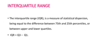
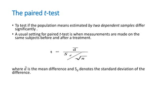
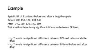
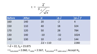
The document defines various statistical measures and types of statistical analysis. It discusses descriptive statistical measures like mean, median, mode, and interquartile range. It also covers inferential statistical tests like the t-test, z-test, ANOVA, chi-square test, Wilcoxon signed rank test, Mann-Whitney U test, and Kruskal-Wallis test. It explains their purposes, assumptions, formulas, and examples of their applications in statistical analysis.


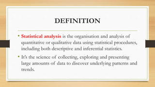
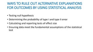
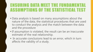
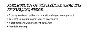
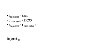
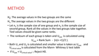
![MEDIAN
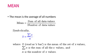
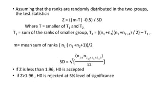
• When all the observations are arranged in ascending or descending
orders of magnitude, the middle one is the median.
• For raw data, If n is the total number of observations, the value of the
[
𝑛+1
2
] th item will be called median .
• if n is the even number, the mean of n/2th item and [
𝑛
2
+ 1] th item
will be median.
Example : Median of given data 10, 20, 30 is
20](https://image.slidesharecdn.com/statisticalanalysis-181011143647/85/Statistical-analysis-10-320.jpg)
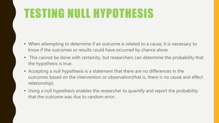
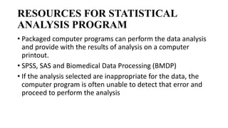
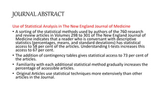
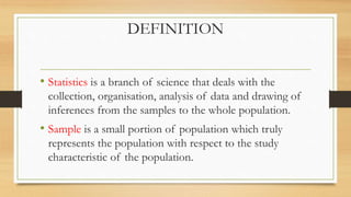
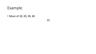
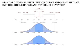
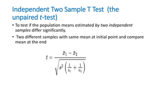
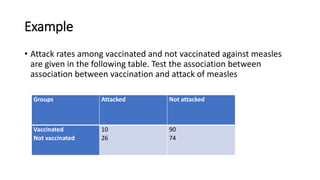
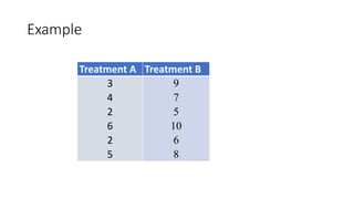
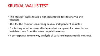
![Example
Interquartile range of following data 30, 20, 40, 60 , 50
• Q1 =[
𝑛+1
4
]th item = 1.5th item = 20+ 0.5 (30-20) = 25
• Q3 = 3[
𝑛+1
4
]th item = 50 +0.5x (60-50) = 55.
• IQR = 30](https://image.slidesharecdn.com/statisticalanalysis-181011143647/85/Statistical-analysis-13-320.jpg)
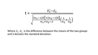
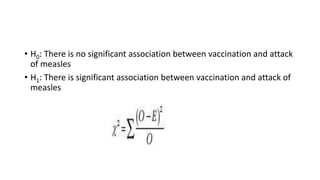
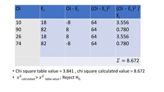
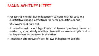
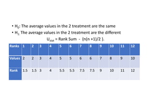
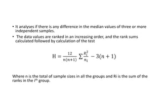
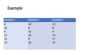
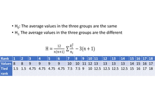
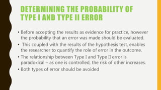
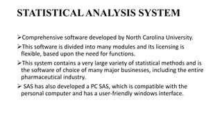
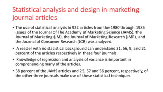
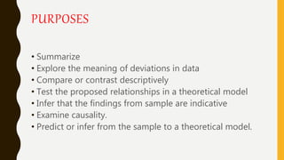
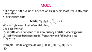
![• H = {12/18x19 [ (45.252 /6 ) + (61.52/6) + (65.52/6 )]} – 3x19
• Hcalculated = 56.99 , 𝑥2
table value = 5.99
• Hstat > 𝑥2
table value ; Reject H0
Sample 1 Rank 1 Sample 2 Rank 2 Sample 3 Rank 3
8
10
9
12
11
13
1.5
7.5
4.75
10
9
12.5
10
9
13
14
9
16
7.5
4.75
12.5
15
4.75
17
13
8
9
13
17
15
12.5
1.5
4.75
12.5
18
16
𝛴 = 45.25 𝛴 = 61.5 𝛴 = 65.25](https://image.slidesharecdn.com/statisticalanalysis-181011143647/85/Statistical-analysis-63-320.jpg)