Download as PDF, PPTX
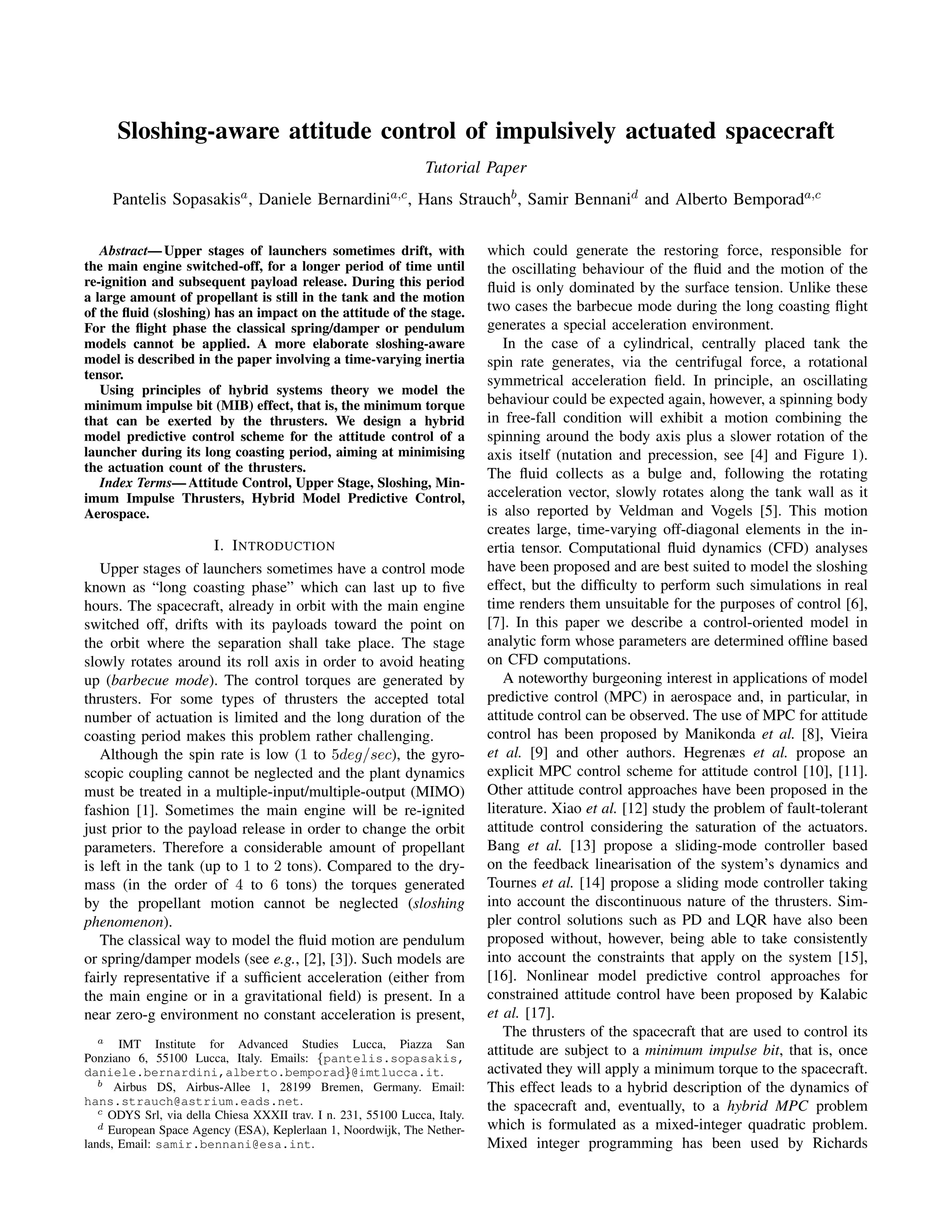
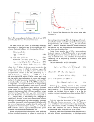


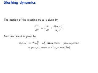
![Ext. Kalman Filter
0 20 40 60 80 100
1
2
3
4
5
6
7
8
9
10
x 10
−4
Time [s]
Stateestimateionerror(norm)
9 / 16](https://image.slidesharecdn.com/ecc15sloshingmpc-150716134550-lva1-app6891/85/Sloshing-aware-MPC-for-upper-stage-attitude-control-13-320.jpg)
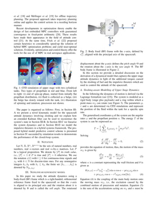
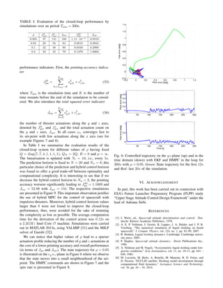
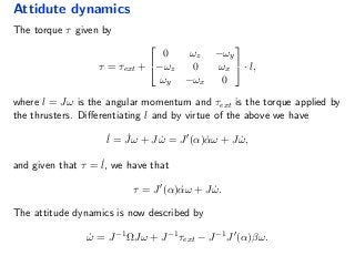
![Minimum impulse effect
Minimum impulse effect: thrusters cannot produce arbitrarily small
torques, thus uk is constrained in
U = [−umax, −umin] ∪ {0} ∪ [umin, umax]
We introduce the binary vectors δ−
k and δ+
k so that1
δ−
k = [uk ≤ −umin],
δ+
k = [uk ≥ umin],
and the auxiliary variable ηk defined as
ηk,i = [δ−
k,i ∨ δ+
k,i] · uk,i
1
Here ≤ and ≥ are element-wise comparison operators.
11 / 16](https://image.slidesharecdn.com/ecc15sloshingmpc-150716134550-lva1-app6891/85/Sloshing-aware-MPC-for-upper-stage-attitude-control-16-320.jpg)
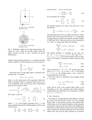
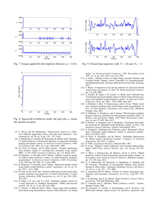
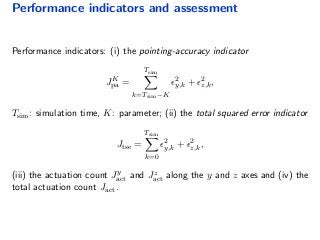
![Minimum impulse effect
To detect thruster activations we use the variable
vk = [δ−
k ∨ δ+
k ]
and we recast the system dynamics as
zk+1 = Azk + Bηk + f,
γk+1 = γk + [ 1 1 1 ] vk,
where γk is the total actuation count up to time k on which we impose:
γk ≤ γmax.
12 / 16](https://image.slidesharecdn.com/ecc15sloshingmpc-150716134550-lva1-app6891/85/Sloshing-aware-MPC-for-upper-stage-attitude-control-17-320.jpg)
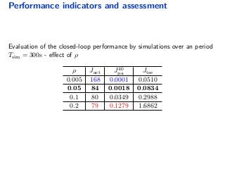
![Hybrid Model Predictive Control
MPC problem2:
P(x0, γ0, A, B, f) : min
πN
VN (πN , γ0)
s.t. x(0) = x0, γ(0) = γ0,
Hybrid dynamics for k ∈ N[0,Nu−1],
Assume U = [−umax, umax] for k ∈ N[Nu,N−1],
where
VN (πN , γ0)= QN zN p + ρ(γN − γ0)
Penalises the tot.
actuation count along
the horizon
+
N−1
k=0
Qzk p + Rηk p
2
Optimisation with respect to the sequence of control actions uk, δk, vk and ηk.
14 / 16](https://image.slidesharecdn.com/ecc15sloshingmpc-150716134550-lva1-app6891/85/Sloshing-aware-MPC-for-upper-stage-attitude-control-20-320.jpg)
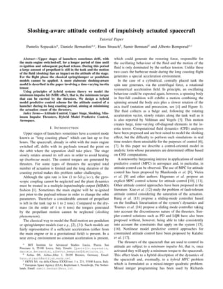
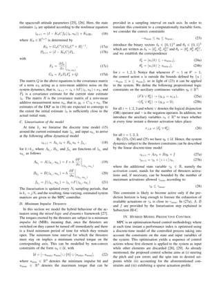
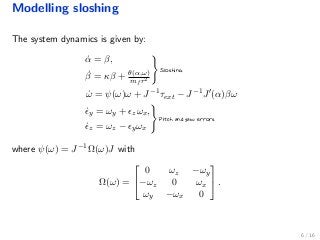
![Simulation results3
−0.2 0 0.2 0.4 0.6 0.8 1 1.2
−0.2
0
0.2
0.4
0.6
0.8
1
1.2
1.4
Pitch error [deg]
Yawerror[deg]
50 100 150 200 250 300
0
0.2
0.4
0.6
0.8
Pitcherror[deg]
50 100 150 200 250 300
0
0.5
1
Yawerror[deg]
Time [s]
0 50 100 150 200 250 300
−6
−4
−2
0
2
4
6
Time [s]
Spinrate[deg/s]
0 50 100 150 200 250 300
0
1000
2000
T
x
0 50 100 150 200 250 300
−2000
0
2000
4000
T
y
0 50 100 150 200 250 300
−2000
0
2000
4000
T
z
Time [s]
3
Simulation parameters: Nu = 8, N = 20, ρ = 0.05
15 / 16](https://image.slidesharecdn.com/ecc15sloshingmpc-150716134550-lva1-app6891/85/Sloshing-aware-MPC-for-upper-stage-attitude-control-21-320.jpg)
![Simulation results
Choosing Nu = 2 we get:
50 100 150 200 250 300
−1
0
1Pitcherror[deg]
50 100 150 200 250 300
−1
0
1
Yawerror[deg]
Time [s]
16 / 16](https://image.slidesharecdn.com/ecc15sloshingmpc-150716134550-lva1-app6891/85/Sloshing-aware-MPC-for-upper-stage-attitude-control-22-320.jpg)

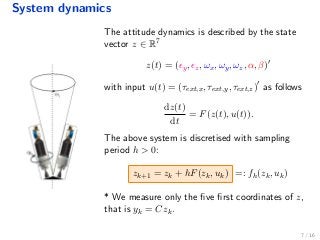
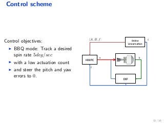
The document discusses a sloshing-aware dynamical model for attitude control of spacecraft utilizing impulsive actuators. It describes methods for state estimation, model linearization, and hybrid model predictive control, emphasizing the effects of sloshing dynamics and constraints of thruster activations. Simulation results demonstrate the control scheme's effectiveness in managing pitch and yaw errors while optimizing actuation counts.