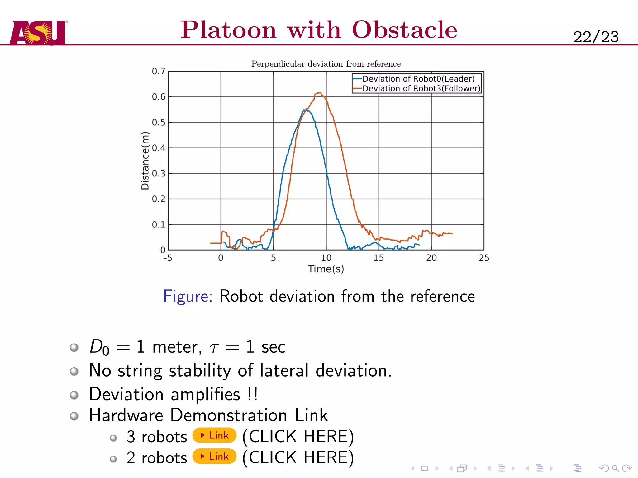
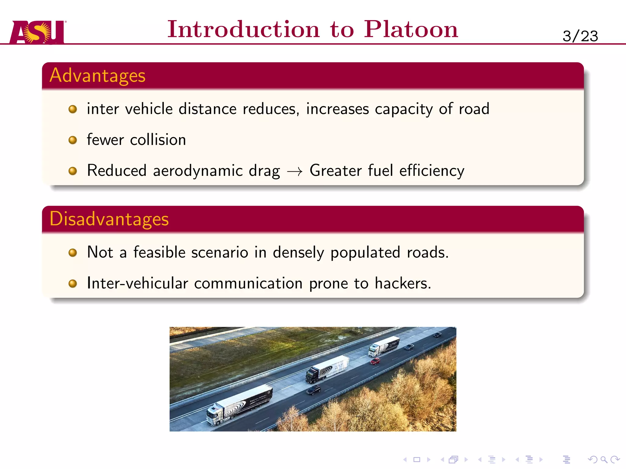
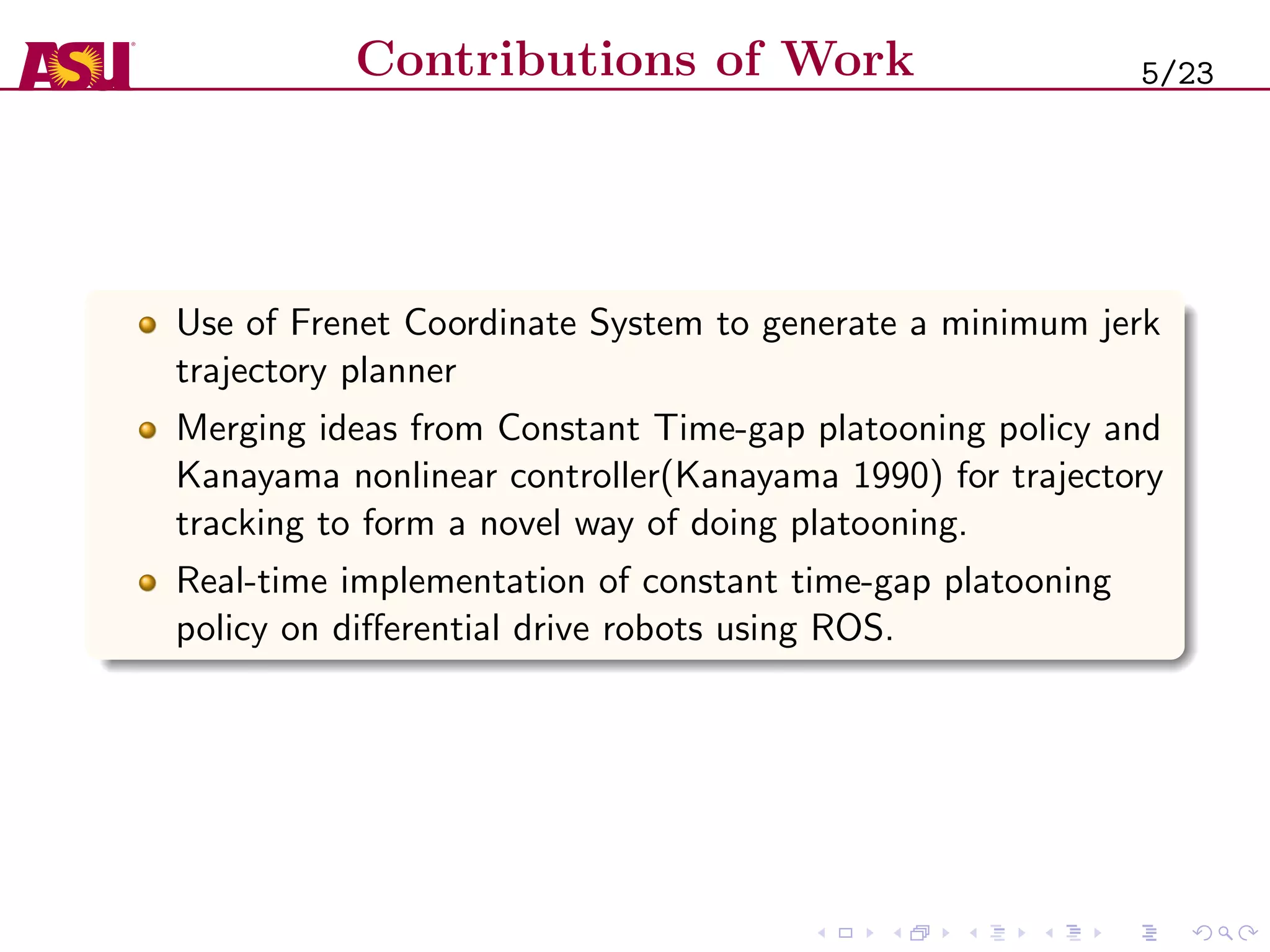
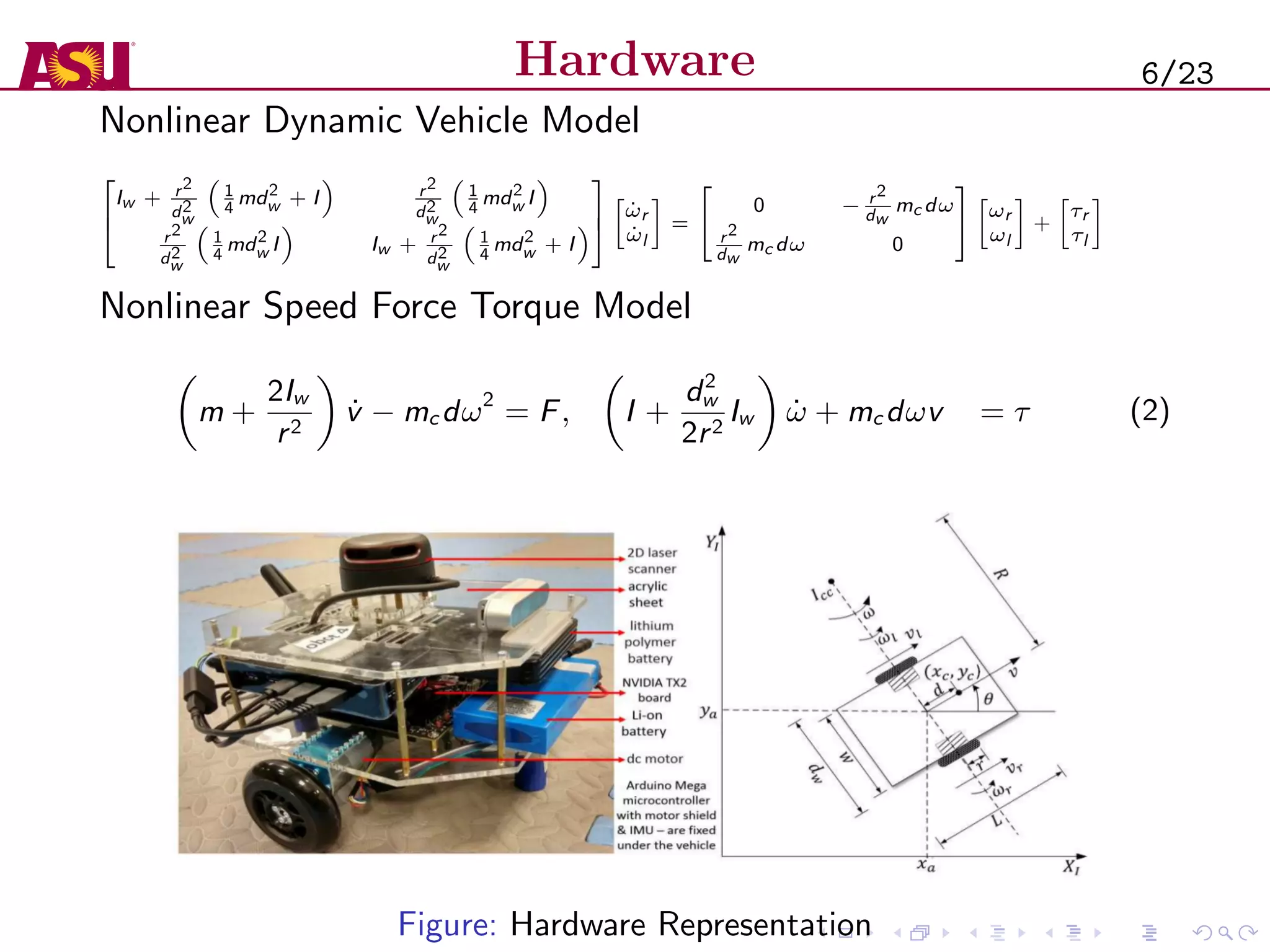
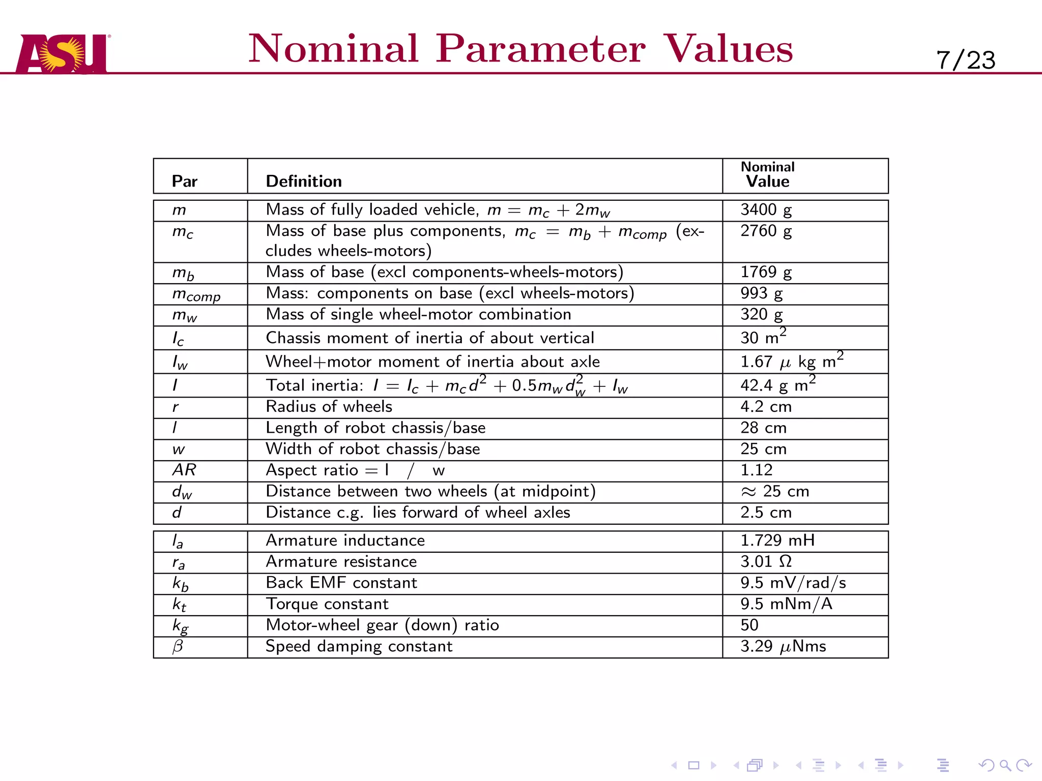
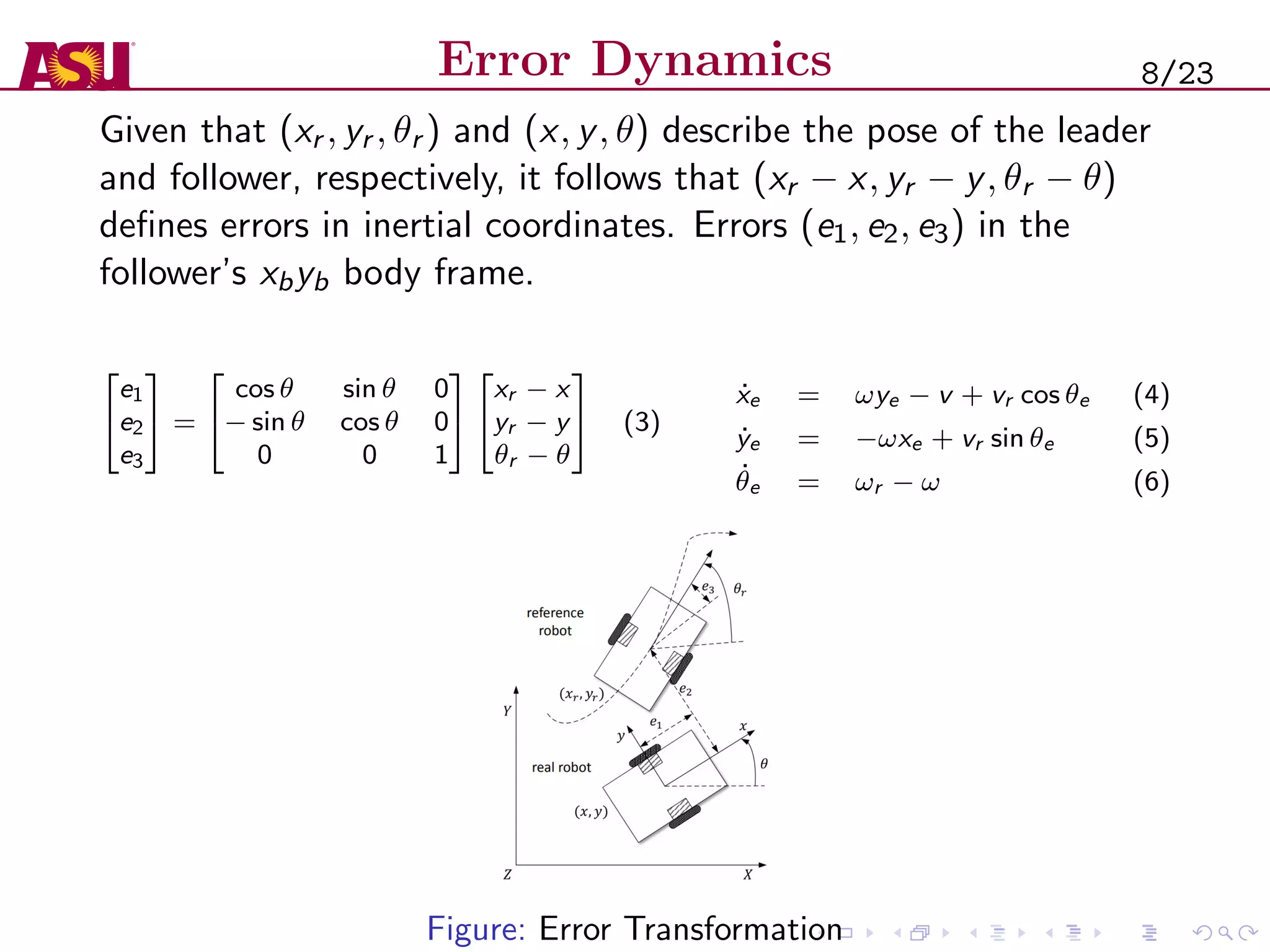
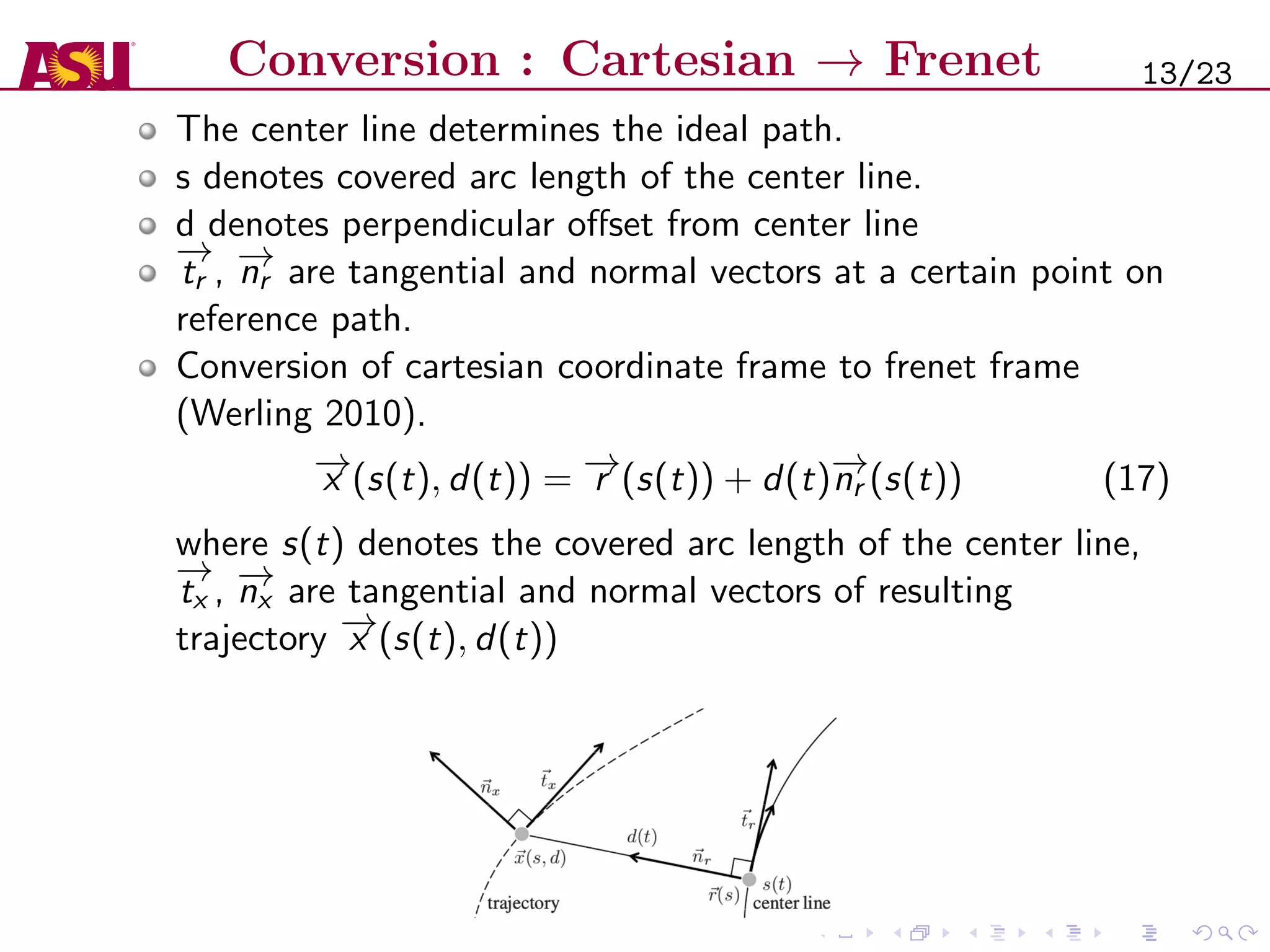
The document presents a final project on controlling nonholonomic robots in a platoon formation using quintic Bezier splines, focusing on algorithm development and hardware implementation. Key contributions include the creation of a minimum jerk trajectory planner and the application of the Kanayama nonlinear controller for real-time trajectory tracking. The work highlights advantages such as improved fuel efficiency and reduced collisions, alongside challenges related to string stability and potential security issues in inter-vehicular communication.

1. Platoon Control of Nonholonomic Robots
using Quintic Bezier Splines
Kaustav Mondal
Department of Electrical Engineering
Arizona State University
Final Project Presentation
EGR 598(Audit)
December 8, 2018
Professor:
Dr. Yan Chen

2. Outline
Introduction to Platoon
Contributions of Work
Hardware representation.
Error Dynamics of Kanayama controller
Inner loop control design
Outer loop control design
Minimum Jerk Trajectory Generation
Trajectory Planner for Leader of Platoon
Trajectory Planner for Follower of Platoon
Localization using Particle Filter
Software and Hardware results.
References
2/23

3. Introduction to Platoon
Advantages
inter vehicle distance reduces, increases capacity of road
fewer collision
Reduced aerodynamic drag → Greater fuel efficiency
Disadvantages
Not a feasible scenario in densely populated roads.
Inter-vehicular communication prone to hackers.
3/23

4. String Stability
G(s) =
δi (s)
δi−1(s)
(1)
The system is string stable if
||G(s)||∞ < 1 (Sheikholeslam, 1990)
The impulse response g(t) does not change sign i.e. g(t) > 0
∀ t ≥ 0 (Rajamani, 1995).
δss for all vehicles have same sign.
Figure: String Unstable Figure: String Stable
4/23

5. Contributions of Work
Use of Frenet Coordinate System to generate a minimum jerk
trajectory planner
Merging ideas from Constant Time-gap platooning policy and
Kanayama nonlinear controller(Kanayama 1990) for trajectory
tracking to form a novel way of doing platooning.
Real-time implementation of constant time-gap platooning
policy on differential drive robots using ROS.
5/23

6. Hardware
Nonlinear Dynamic Vehicle Model



Iw + r2
d2
w
1
4
md2
w + I r2
d2
w
1
4
md2
w I
r2
d2
w
1
4
md2
w I Iw + r2
d2
w
1
4
md2
w + I



˙ωr
˙ωl
=


0 − r2
dw
mc dω
r2
dw
mc dω 0

 ωr
ωl
+
τr
τl
Nonlinear Speed Force Torque Model
m +
2Iw
r2
˙v − mc dω2
= F, I +
d2
w
2r2
Iw ˙ω + mc dωv = τ (2)
Figure: Hardware Representation
6/23

7. Nominal Parameter Values
Par Definition
Nominal
Value
m Mass of fully loaded vehicle, m = mc + 2mw 3400 g
mc Mass of base plus components, mc = mb + mcomp (ex-
cludes wheels-motors)
2760 g
mb Mass of base (excl components-wheels-motors) 1769 g
mcomp Mass: components on base (excl wheels-motors) 993 g
mw Mass of single wheel-motor combination 320 g
Ic Chassis moment of inertia of about vertical 30 m2
Iw Wheel+motor moment of inertia about axle 1.67 µ kg m2
I Total inertia: I = Ic + mc d2
+ 0.5mw d2
w + Iw 42.4 g m2
r Radius of wheels 4.2 cm
l Length of robot chassis/base 28 cm
w Width of robot chassis/base 25 cm
AR Aspect ratio = l / w 1.12
dw Distance between two wheels (at midpoint) ≈ 25 cm
d Distance c.g. lies forward of wheel axles 2.5 cm
la Armature inductance 1.729 mH
ra Armature resistance 3.01 Ω
kb Back EMF constant 9.5 mV/rad/s
kt Torque constant 9.5 mNm/A
kg Motor-wheel gear (down) ratio 50
β Speed damping constant 3.29 µNms
7/23

8. Error Dynamics
Given that (xr , yr , θr ) and (x, y, θ) describe the pose of the leader
and follower, respectively, it follows that (xr − x, yr − y, θr − θ)
defines errors in inertial coordinates. Errors (e1, e2, e3) in the
follower’s xbyb body frame.


e1
e2
e3

 =


cos θ sin θ 0
− sin θ cos θ 0
0 0 1




xr − x
yr − y
θr − θ

 (3)
˙xe = ωye − v + vr cos θe (4)
˙ye = −ωxe + vr sin θe (5)
˙θe = ωr − ω (6)
Figure: Error Transformation
8/23

9. Inner Loop Control Design
Assuming the plant P[e→ωr,l ] to be decoupled,
Kinner = kI2×2
where k = g(s+z)
s
b
s+b , g = 5, z = 10, b = 200.
Figure: Inner-Loop System
Figure: Sensitivities So = Si , To = Ti for Coupled P[e→[v,ω]]
9/23

10. Outer Loop Control Design
Feedforward Term
vff
ωff
=
vr cos e3
ωr
(7)
Feedback Controller (Kanayama
1990)
vfb
ωfb
=
−kx xe
−vr ky kθye − vr kθ sin θe
(8)
Figure: Outer-Loop System
Substituting feedforward and feedback terms, the new error
dynamics :
˙xe = −kx xe + ωye (9)
˙ye = −ωxe + vr sin θe (10)
˙θe = −vr kθky ye − vr kθ sin θe (11)
10/23

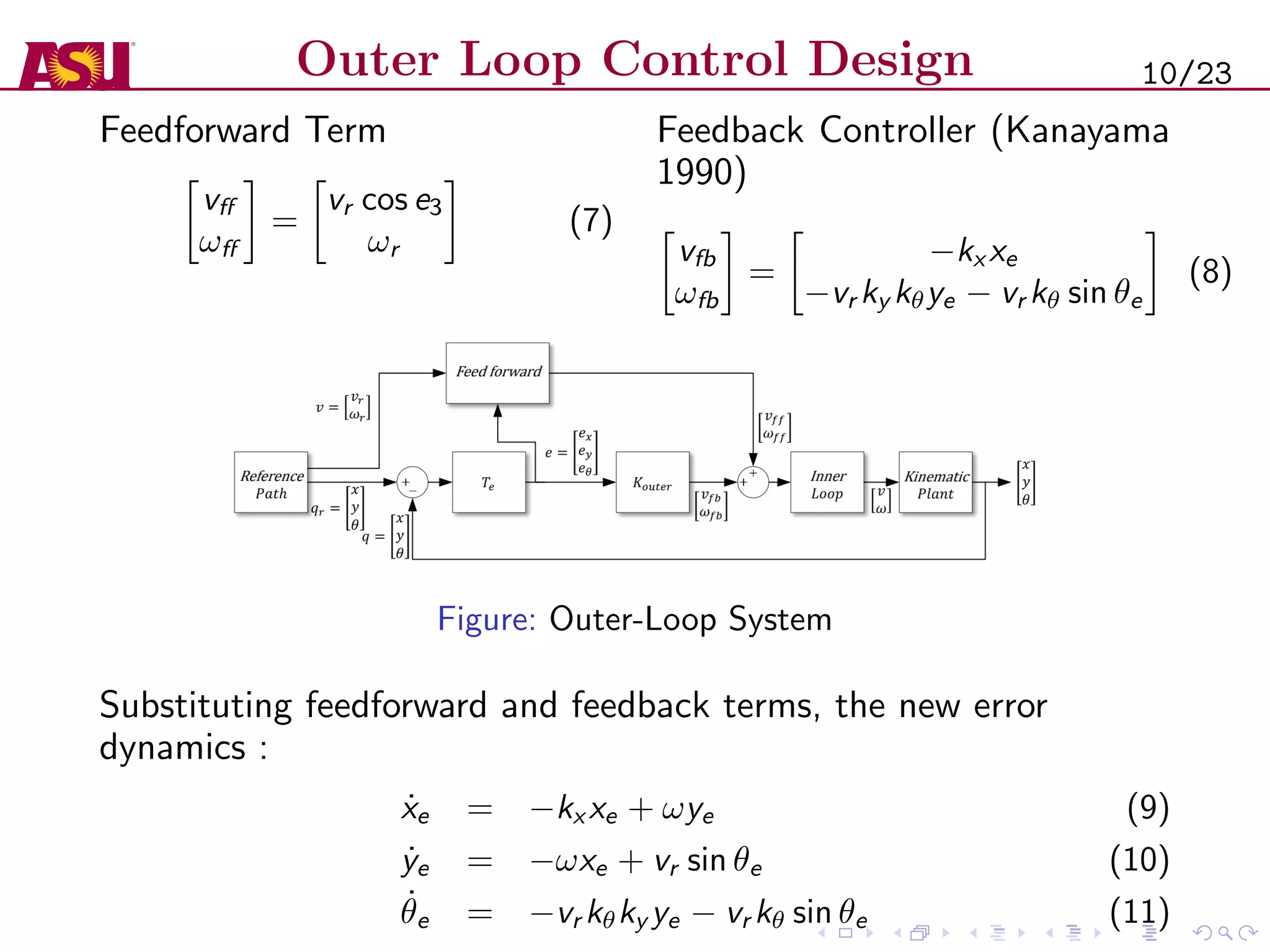
11. Outer Loop Control Design
Linearized error dynamics near qe = [ xe ye θe ]T = 0:
˙qe = Aqe A =


−kx ωr 0
−ωr 0 vr
0 −vr kθky −vr kθ

 (12)
Φ(s) = det(sI − A) = s3 + a2s2 + a1s + ao where
a2 = kx + vr kθ,
a1 = v2
r ky kθ + vr kx kθ + ω2
r ,
ao = vr ω2
r kθ + v2
r kx ky kθ.
A is hurwitz if a2a1 > ao.
vr > 0, kx , ky , kθ > 0 (Assumption)
kx = 0.75, ky = 4, kth = 4.5 (Hardware Implementation)
If ˙vr and ˙ωr are sufficiently small (Low, 2012), the equilibrium
qe = 0 is locally exponentially stable. Lyapunov analysis and
Barlabat’s Lemma have been used.
11/23

12. Minimum Jerk Trajectory Generation
x∗
(t) = argmin
x(t)
T
0
L(
...
x , ¨x, ˙x, x, t)dt = argmin
x(t)
T
0
...
x (t)dt (13)
We solve the Euler Lagrange Equation:
∂L
∂x
−
d
dt
(
∂L
∂ ˙x
) +
d2
dt2
(
∂L
∂¨x
) −
d3
dt3
(
∂L
∂x(3)
) = 0 (14)
x(t) =
∞
n=0
αntn
(15)
x∗(t) = α0 + α1t + α2t2 + α3t3 + α4t4 + α5t5
6 coefficients, 6 tunable parameters, 6 boundary conditions
Initial Condition [xi , ˙xi , ¨xi ], Final Condition [xf , ˙xf , ¨xf ]
α0 = xi , α1 = ˙xi , α2 = 1
2 ¨xi


T3
T4
T5
3T2
4T3
5T4
6T 12T2
20T3

 ×


α3
α4
α5

 =


xf − (xi + ˙xi T + 1
2
¨xT2
)
˙xf − ( ˙xi + ¨xi T)
¨xf − ¨xi

 (16)
12/23

13. Conversion : Cartesian → Frenet
The center line determines the ideal path.
s denotes covered arc length of the center line.
d denotes perpendicular offset from center line
−→
tr , −→nr are tangential and normal vectors at a certain point on
reference path.
Conversion of cartesian coordinate frame to frenet frame
(Werling 2010).
−→x (s(t), d(t)) = −→r (s(t)) + d(t)−→nr (s(t)) (17)
where s(t) denotes the covered arc length of the center line,
−→
tx , −→nx are tangential and normal vectors of resulting
trajectory −→x (s(t), d(t))
13/23

14. Generation of Trajectories
Generation of 1D trajectories for s(arc length) and d(deviation).
argmin
s(t)
Cs (t)
s.t. t ∈ [t1, t2],
where
Cs (t) = k1
t2
t1
...
s (t)dt + k2t2 +
k3(sref (t2) − s(t2))2
t1 = t0
t2 = t0 + T
Jerk optimal trajectory from
[si , ˙si , ¨si , t1] → [starget , ˙starget , ¨starget , t2]
argmin
d(t)
Cd (t)
s.t. t ∈ [t1, t2],
where
Cd (t) = k4
t0+T
t0
...
d (t)dt +
k5t2 + k6(dref (t2) − d(t2))2
t1 = t0
t2 = t0 + T
Jerk optimal trajectory from
[di , ˙di , ¨di , t1] → [dtarget , 0, 0, t2]
Neglecting trajectories which intersect with obstacles, we select the
trajectory with the minimum Cs(t) + Cd (t).
14/23

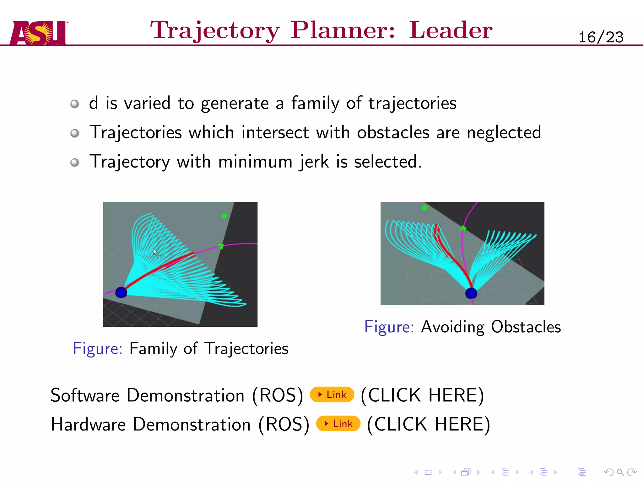
15. Trajectory Planner: Leader
Trajectory Planner for Leader
Velocity keeping trajectory planner.
[s0, ˙s0, ¨s0, t1] → [ ˙starget , ¨starget , t2]
[d0, ˙d0, ¨d0, t1] → [d, 0, 0, t2] where dtarget − < d < dtarget +
Minimize the cost functional
argmin
s(t)
k1
t2
t1
...
s (t)dt + k2t2 + k3( ˙starget (t2) − ˙s(t2))2
s.t. t ∈ [t1, t2],
argmin
d(t)
k4
t2
t1
...
d (t)dt + k4t2 + k6(dtarget (t2) − d(t2))2
s.t. t ∈ [t1, t2],
s∗(t) = 4
n=0 αntn (Quartic Polynomial)
d∗(t) = 5
n=0 αntn (Quintic Polynomial)
Target point is tracked by leader using Kanayama nonlinear
controller(Kanayama 1990).
15/23

16. Trajectory Planner: Leader
d is varied to generate a family of trajectories
Trajectories which intersect with obstacles are neglected
Trajectory with minimum jerk is selected.
Figure: Family of Trajectories
Figure: Avoiding Obstacles
Software Demonstration (ROS) Link (CLICK HERE)
Hardware Demonstration (ROS) Link (CLICK HERE)
16/23

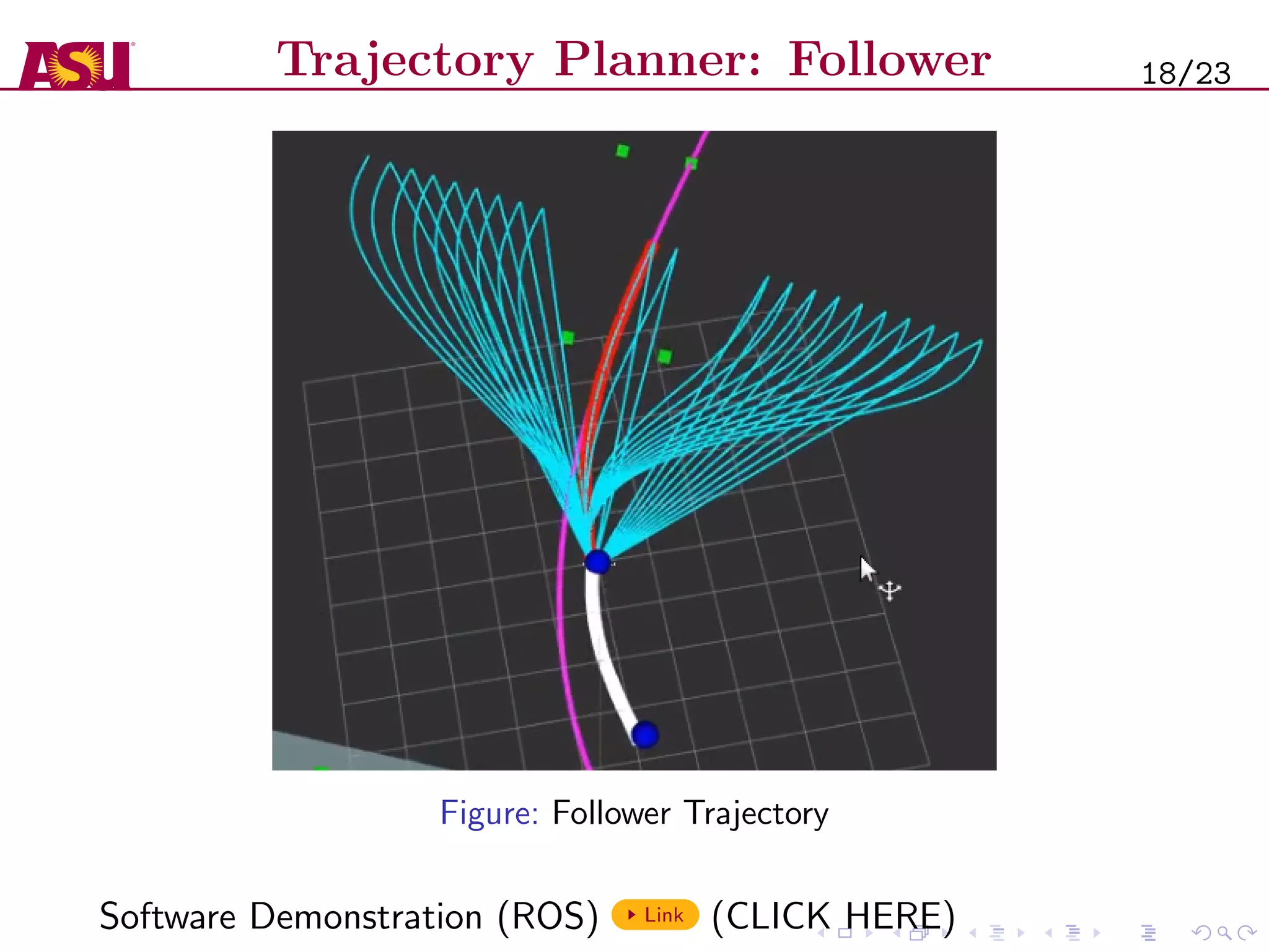
17. Trajectory Planner: Follower
Trajectory Planner for follower
Use of Constant time-gap law for safety.
[starget, ˙starget, ¨starget, t1] → [slv , ˙slv , ¨slv , t2]
starget = slv − (D0 + τ ˙slv )
˙starget = ˙slv − τ ¨slv
¨starget = ¨slv
[slv , ˙slv , ¨slv , t2] represents position of Leader.
[starget, ˙starget, ¨starget, t1] represents desired position of Follower.
D0 is the standstill distance between robots
τ is the time-constant of the Constant time-gap law.
[dtarget, ˙dtarget, ¨dtarget, t1] → [dlv , 0, 0, t2]
dv is the perpendicular deviation from reference trajectory.
The target point is tracked by follower using Kanayama
Controller(Kanayama 1990).
17/23

18. Trajectory Planner: Follower
Figure: Follower Trajectory
Software Demonstration (ROS) Link (CLICK HERE)
18/23

19. Localization
Adaptive Monte Carlo Localization (http://wiki.ros.org/amcl)
Localizes against pre-existing map in 2D space.
Map generated using SLAM (http://wiki.ros.org/gmapping)
Kullback Leibler divergence (KLD Sampling)
Variable Particle Size
Sample size is proportional to error between odometry position and
sample based position.
Smaller sample size when particles have converged.
Use of Odometry data for Prediction step.
Use of Lidar Scan data for Update step.
Figure: Uncertain Initial Position Figure: Updated Position
19/23

20. Constant Timegap Policy (τ = 1 sec)
Platoon of 3 robots
D0 = 1 meter, τ = 1 sec
Inter robot distance
converges to 1 meter at
standstill.
Inter robot distance
amplifies down the platoon
Velocity amplifies during
transients.
No String Stability.
Hardware Demonstration
Link Link (CLICK HERE)
20/23

21. Constant Timegap Policy (τ = 2 sec)
Platoon of 3 robots
D0 = 1 meter, τ = 2 sec
Inter robot distance
converges to 1 meter at
standstill.
Inter robot distance
amplifies down the platoon
Velocity amplifies during
transients.
No String Stability.
21/23

22. Platoon with Obstacle
Figure: Robot deviation from the reference
D0 = 1 meter, τ = 1 sec
No string stability of lateral deviation.
Deviation amplifies !!
Hardware Demonstration Link
3 robots Link (CLICK HERE)
2 robots Link (CLICK HERE)
22/23

23. References
S. Sheikholeslam, C.A. Desoer, Longitudinal Control of a
Platoon of Vehicles with no Communication of Lead Vehicle
Information: A System Level Study, IEEE transactions on
Vehicle Technology, Vol. 42, No.4, 1993.
S. Sheikholeslam, C.A. Desoer, Longitudinal Control of
Platoons, American Control Conference(ACC), pp. 291-296,
IEEE, 1990.
R. Rajamani, Vehicle Dynamics and Control, Springer Science,
1995.
Y. Kanayama, Y. Kimura, F. Miyazaki, T. Noguchi, A stable
tracking control method for an autonomous mobile robot,
1990.
C. Low, A trajectory tracking control scheme design for
nonholonomic wheeled mobile robots with low-level control
systems, 2012 IEEE 51st Annual Conf on Decision and
Control (CDC), pp. 536543, IEEE, 2012.
23/23