Download to read offline
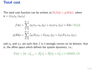
![Applications
Microgrids [Hans et al. ’15]
Drinking water networks [Sampathirao et al. ’15]
HVAC [Long et al. ’13, Zhang et al. ’13, Parisio et al. ’13]
Financial systems [Patrinos et al. ’11, Bemporad et al., ’14]
Chemical process [Lucia et al. ’13]
Distillation column [Garrido and Steinbach, ’11]
1 / 28](https://image.slidesharecdn.com/cdc2015-151218061929/85/Distributed-solution-of-stochastic-optimal-control-problem-on-GPUs-2-320.jpg)
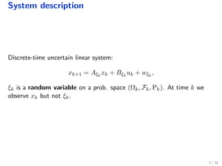
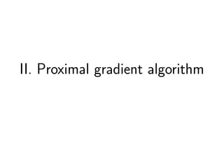
![Stochastic optimal control problem
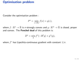
Optimisation problem:
V (p) = min
π={uk}k=N−1
k=0
E Vf (xN , ξN ) +
N−1
k=0
k(xk, uk, ξk) ,
s.t x0 = p,
xk+1 = Aξk
xk + Bξk
uk + wξk
,
where:
E[·]: conditional expectation wrt the product probability measure
6 / 28](https://image.slidesharecdn.com/cdc2015-151218061929/85/Distributed-solution-of-stochastic-optimal-control-problem-on-GPUs-9-320.jpg)
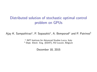
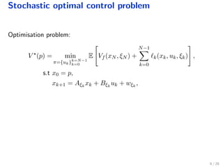
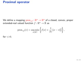
![Stochastic optimal control problem
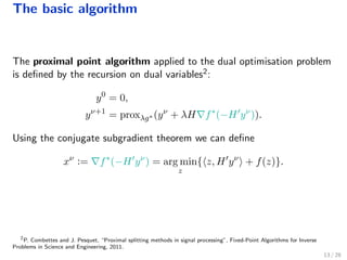
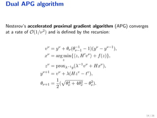
Optimisation problem:
V (p) = min
π={uk}k=N−1
k=0
E Vf (xN , ξN ) +
N−1
k=0
k(xk, uk, ξk) ,
s.t x0 = p,
xk+1 = Aξk
xk + Bξk
uk + wξk
,
where:
E[·]: conditional expectation wrt the product probability measure
Casual policy uk = ψk(p,ξξξk−1), with ξξξk = (ξ0, ξ1, . . . , ξk)
6 / 28](https://image.slidesharecdn.com/cdc2015-151218061929/85/Distributed-solution-of-stochastic-optimal-control-problem-on-GPUs-10-320.jpg)
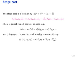
![Stochastic optimal control problem
Optimisation problem:
V (p) = min
π={uk}k=N−1
k=0
E Vf (xN , ξN ) +
N−1
k=0
k(xk, uk, ξk) ,
s.t x0 = p,
xk+1 = Aξk
xk + Bξk
uk + wξk
,
where:
E[·]: conditional expectation wrt the product probability measure
Casual policy uk = ψk(p,ξξξk−1), with ξξξk = (ξ0, ξ1, . . . , ξk)
and Vf can encode constraints
6 / 28](https://image.slidesharecdn.com/cdc2015-151218061929/85/Distributed-solution-of-stochastic-optimal-control-problem-on-GPUs-11-320.jpg)
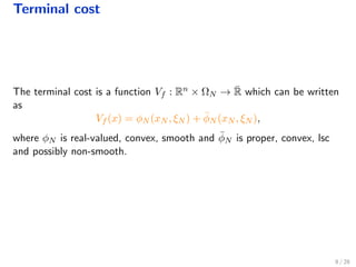
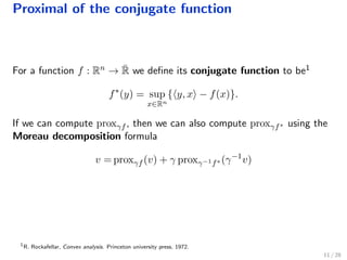
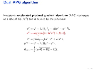
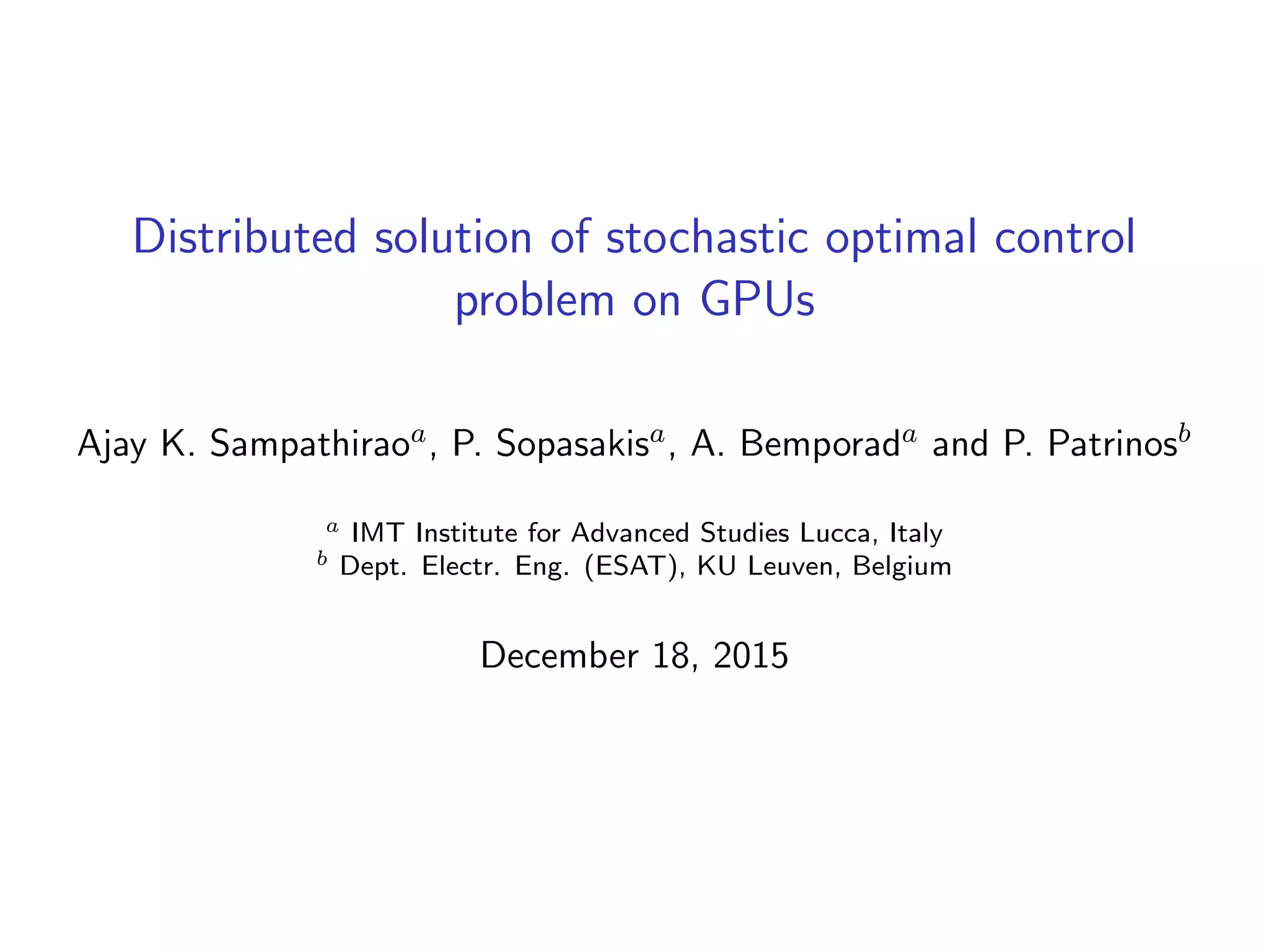
![Computation of the dual gradient
Factor step:
Performed once
Parallelisable
For time-invariant problems,
can be performed once offline
Algorithm 1 Solve step
qi
N ← yi
N , ∀i ∈ N[1,µ(N)], %Backward substitution
for k = N − 1, . . . , 0 do
for i ∈ µ(k) do {in parallel}
ui
k ← Φi
kyi
k + j∈child(k,i) Θ
j
k
q
j
k+1
+ σi
k
qi
k ← Di
k yi
k + j∈child(k,i) Λ
j
k
q
j
k+1
+ ci
k
end for
end for
x1
0 = p, %Forward substitution
for k = 0, . . . , N − 1 do
for i ∈ µ(k) do {in parallel}
ui
k ← Ki
kxi
k + ui
k
for j ∈ child(k, i) do {in parallel}
x
j
k+1
← A
j
k
xi
k + B
j
k
ui
k + w
j
k
end for
end for
end for
19 / 28](https://image.slidesharecdn.com/cdc2015-151218061929/85/Distributed-solution-of-stochastic-optimal-control-problem-on-GPUs-28-320.jpg)
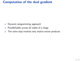
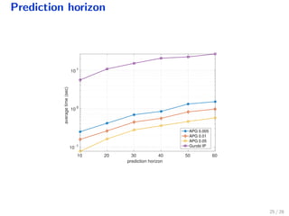
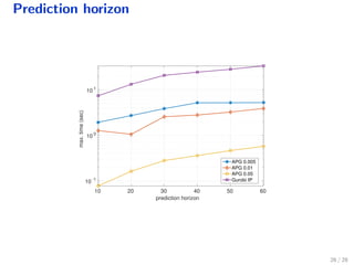


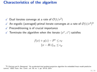
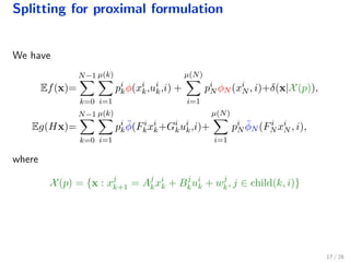
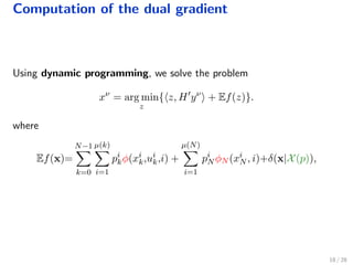
The document discusses a distributed solution for a stochastic optimal control problem using GPUs, highlighting the advantages of accelerated proximal gradient algorithms for solving complex control challenges across various applications like microgrids and drinking water networks. It includes a formulation of the optimization problem, details about the algorithm's implementation and performance, and presents simulation results demonstrating significant speed improvements compared to traditional methods like interior-point solvers. The findings indicate a substantial reduction in runtime, emphasizing the efficacy of GPU-based solutions for large-scale stochastic control systems.