Downloaded 411 times


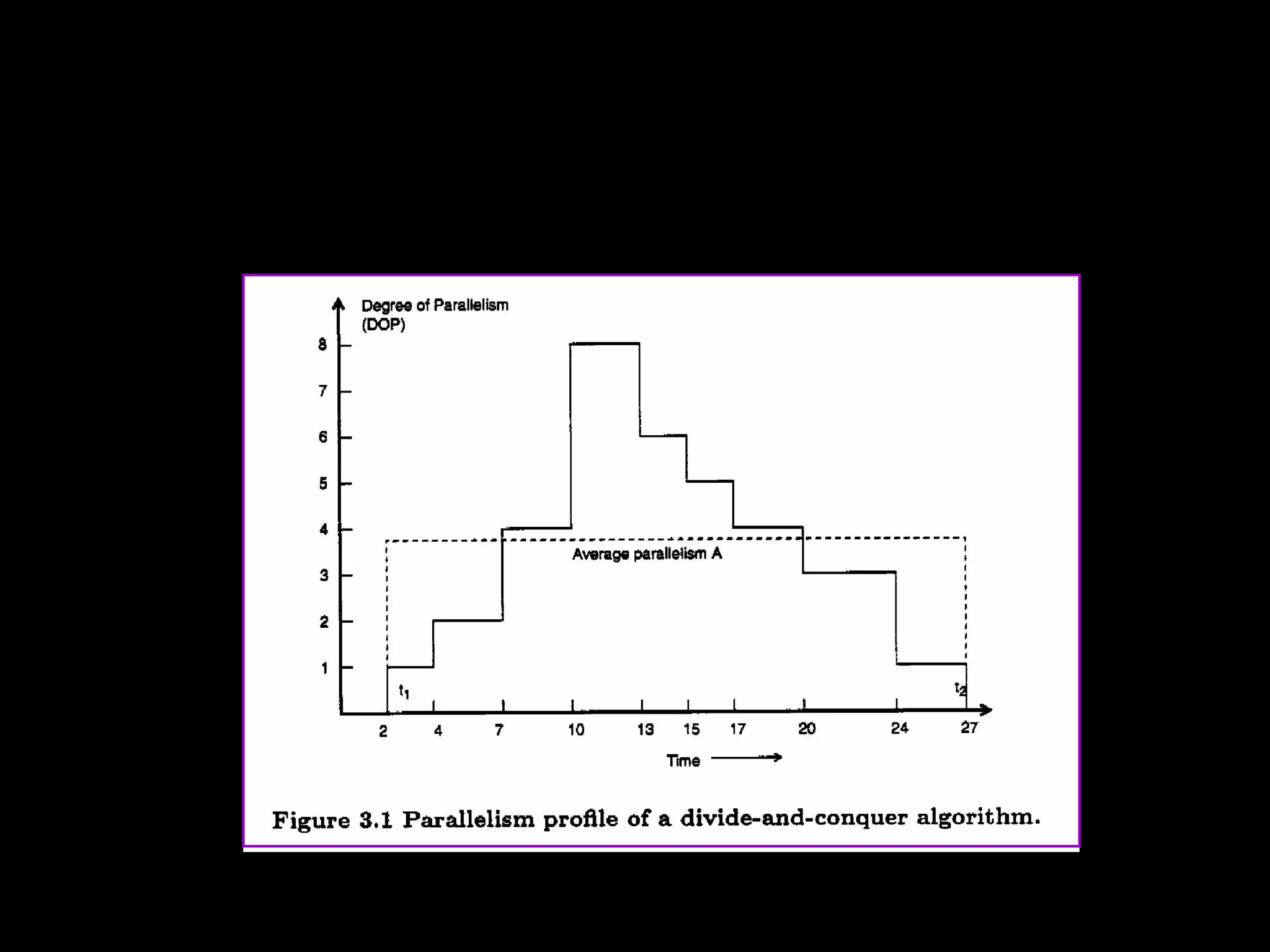


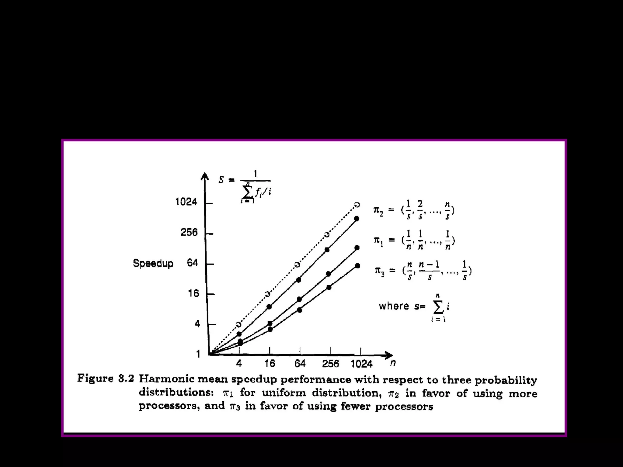


This chapter discusses principles of scalable performance for parallel systems. It covers performance measures like speedup factors and parallelism profiles. The key principles discussed include degree of parallelism, average parallelism, asymptotic speedup, efficiency, utilization, and quality of parallelism. Performance models like Amdahl's law and isoefficiency concepts are presented. Standard performance benchmarks and characteristics of parallel applications and algorithms are also summarized.