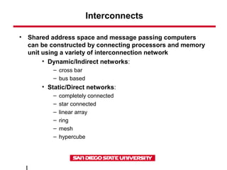
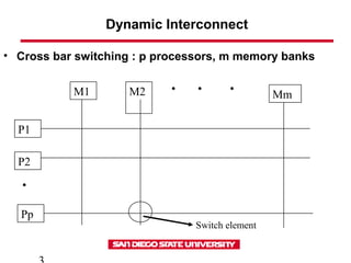
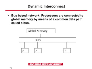
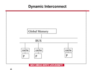
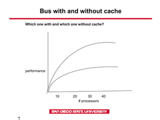
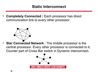
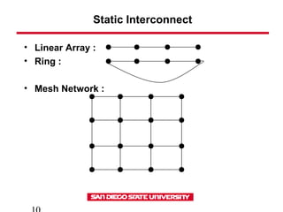
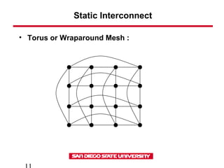
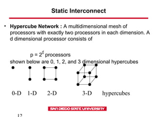
SlideShare a Scribd company logo
Interconnects
• Shared address space and message passing computers
can be constructed by connecting processors and memory
unit using a variety of interconnection network
• Dynamic/Indirect networks:
– cross bar
– bus based
• Static/Direct networks:
– completely connected
– star connected
– linear array
– ring
– mesh
– hypercube
More on Interconnects
• Dynamic Interconnect: Communication links are
connected to one another dynamically by the
switching elements to establish path among
processors and memory banks. Normally used for
share memory address space computers.
• Static/Direct Interconnect : Consists of point to
point communication links among processors.
Typically used for message passing computers.
Dynamic Interconnect
• Cross bar switching : p processors, m memory banks
M1 M2 Mm
P1
P2
Pp
. . .
.
Switch element
Dynamic Interconnect
• Cross Bar switch is a non blocking network i.e.
connection of a processor to a memory bank
does not block the connection of any other
processor to any other memory bank.
Total # of switching elements required is
f(p*m) = approx f(p*p) (assuming p = m)
As p complexity of switching network f(p*p)
Cross bar switches are not scalable in terms of
cost.
Dynamic Interconnect
• Bus based network: Processors are connected to
global memory by means of a common data path
called a bus.
Global Memory
BUS
P P P
Dynamic Interconnect
Global Memory
BUS
P P P
cache cache cache
Bus with and without cache
10 20 30 40
# processors
performance
Which one with and which one without cache?
Dynamic Interconnect
• Bus based network
• Simplicity of construction
• Provides uniform access to shared memory
• Bus can carry limited amount of data between the
memory and processors
• As the number of processors increases each
processor spends more time waiting for memory
access while the bus is used by other processor
Static Interconnect
• Completely Connected : Each processor has direct
communication link to every other processor
• Star Connected Network : The middle processor is the
central processor. Every other processor is connected to it.
Counter part of Cross Bar switch in Dynamic interconnect.
Static Interconnect
• Linear Array :
• Ring :
• Mesh Network :
Static Interconnect
• Torus or Wraparound Mesh :
Static Interconnect
• Hypercube Network : A multidimensional mesh of
processors with exactly two processors in each dimension. A
d dimensional processor consists of
p = 2
d
processors
shown below are 0, 1, 2, and 3 dimensional hypercubes
0-D 1-D 2-D 3-D hypercubes
More on Static Interconnects
• Diameter : Maximum distance between any two processors
in the network. (the distance between two processors is
defined as the shortest path, in terms of links, between
them). This relates to communication time. Diameter for
completely connected network is 1, for star network is 2, for
ring is p/2 (for p even processors)
• Connectivity: This is a measure of the multiplicity of paths
between any two processors (# arcs that must be removed
to break into two). High connectivity is desired since it
lowers contention for communication resources.
Connectivity is 1 for linear array, 1 for star, 2 for ring, 2 for
mesh, 4 for torus.
More on Static Interconnects
• Bisection width: Minimum # of communication links that have to be
removed to partition the network into two equal halves. Bisection width is
2 for ring, sq. root(p) for mesh with p (even) processors, p/2 for
hypercube, (p*p)/4 for completely connected (p even).
• Channel width: # of physical wires in each communication link
• Channel rate: Peak rate at which a single physical wire link can deliver
bits
• Channel BW : Peak rate at which data can be communicated between
the ends of a communication link ( = (channel width) * (channel rate) )
• Bisection BW : Minimum volume of communication allowed between
any 2 halves of the network with equal # of procs
( = (bisection width) * (channel BW) )
Communication Time Modeling
• Tcomm = Nmsg * Tmsg
Nmsg = # of non overlapping messages
Tmsg = time for one point to point communication
L = length of message ( for e.g in words)
Tmsg = ts + tw * L
latency = ts = startup time (size independent)
tw = asymptotic time per word (1/BW)
Performance and Scalability Terms
• Serial runtime(Ts): Time elapsed between the begining
and the end of execution of a sequential program
• Parallel runtime(Tn): Time that elapses from the moment
that a parallel computer starts to execute to the moment
that the last processor finishes execution.
• Speedup(S): Ratio of the serial runtime of the best
sequential algorithm for solving a problem to the time taken
by the parallel algorithm to solve the same problem on N
processors.
Ts = serial time
Tn = parallel time on N processors
S = Ts/Tn
Performance and Scalability Terms
• Efficiency: Measure of the fraction of time for which a
processor is usefully employed. Defined as the ratio of
speedup to the number of processor. E = S/N
• Amdahl’s law : discussed before
• Scalability : An algorithm is scalable if the level of
parallelism increases at least linearly with the problem size.
An architecture is scalable if it continues to yield the same
performance per processor, albeit used on a larger problem
size, as the # of processors increases. Algorithm and
architecture scalability are important since they allow a user
to solve larger problems in the same amount of time by
buying a parallel computer with more processors.
Performance and Scalability Terms
• Superlinear speedup: In practice a speedup greater than N
(on N processors) is called superlinear speedup. This is
observed due to
1. Non optimal sequential algorithm
2. Sequential problem may not fit in one processor’s main
memory and require slow secondary storage, whereas on
multiple processors problem fits in main memory of N
processors
Sources of Parallel Overhead
• Interprocessor communication: Time to transfer data
between processors is usually the most significant source of
parallel processing overhead.
• Load imbalance: In some parallel applications it is
impossible to equally distribute the subtask workload to
each processor. So at some point all but one processor
might be done and waiting for one processor to complete.
• Extra computation: Sometime the best sequential
algorithm is not easily parallelizable and one is forced to use
a parallel algorithm based on a poorer but easily
parallelizable sequential algorithm. Sometimes repetitive
work is done on each of the N processors instead of
send/recv, which leads to extra computation.
CPU Performance Comparison
MIPS = millions of instructions per second
= IC / (execution time in second* 106
)
= clock rate / (CPI * 106
)
(IC = Instruction count for a program;
CPI = CPU clock cycles for a program/ IC)
MIPS is not an accurate measure for computing performance
among computers :
• MIPS is dependent on the instruction set, making it difficult
to compare MIPS of computers with different instruction set
• MIPS varies between programs on the same computer
• MIPS can vary inversely to performance
CPU Performance Comparison
# of floating point operations in a program
MFLOPS = ----------------------------------------------------------------
execution time in seconds * 106
• MFLOPS (Millions of Floating Point Operations per Second)
are dependent on the machine and on the program ( same
program running on different computers would execute a
different # of instructions but the same # of FP operations)
• MFLOPS is also not a consistent and useful measure of
performance because
– Set of FP operations is not consistent across machines e.g.
some have divide instructions, some don’t
– MFLOPS rating for a single program cannot be generalized
to establish a single performance metric for a computer
CPU Performance Comparison
• Execution time is the principle measure of
performance
• Unlike execution time, it is tempting to
characterize a machine with a single MIPS, or
MFLOPS rating without naming the program,
specifying I/O, or describing the version of OS
and compilers

More Related Content

What's hot

Inter process communication
Inter process communicationInter process communication
Inter process communication
Gift Kaliza
 
Lecturre 07 - Chapter 05 - Basic Communications Operations
Lecturre 07 - Chapter 05 - Basic Communications  OperationsLecturre 07 - Chapter 05 - Basic Communications  Operations
Lecturre 07 - Chapter 05 - Basic Communications Operations
National College of Business Administration & Economics ( NCBA&E)
 
Lecture 05 - Chapter 3 - Models of parallel computers and interconnections
Lecture 05 - Chapter 3 - Models of parallel computers and  interconnectionsLecture 05 - Chapter 3 - Models of parallel computers and  interconnections
Lecture 05 - Chapter 3 - Models of parallel computers and interconnections
National College of Business Administration & Economics ( NCBA&E)
 
Solution(1)
Solution(1)Solution(1)
Solution(1)
Gopi Saiteja
 
Communication model of parallel platforms
Communication model of parallel platformsCommunication model of parallel platforms
Communication model of parallel platforms
Syed Zaid Irshad
 
Chap2 slides
Chap2 slidesChap2 slides
Chap2 slides
BaliThorat1
 
Lecture 06 - Chapter 4 - Communications in Networks
Lecture 06 - Chapter 4 - Communications in NetworksLecture 06 - Chapter 4 - Communications in Networks
Lecture 06 - Chapter 4 - Communications in Networks
National College of Business Administration & Economics ( NCBA&E)
 
Lecture 2 more about parallel computing
Lecture 2   more about parallel computingLecture 2   more about parallel computing
Lecture 2 more about parallel computing
Vajira Thambawita
 
IPC
IPCIPC
Lecture 7 cuda execution model
Lecture 7   cuda execution modelLecture 7   cuda execution model
Lecture 7 cuda execution model
Vajira Thambawita
 
Chap4 slides
Chap4 slidesChap4 slides
Chap4 slides
BaliThorat1
 
Lecture 04 chapter 2 - Parallel Programming Platforms
Lecture 04  chapter 2 - Parallel Programming PlatformsLecture 04  chapter 2 - Parallel Programming Platforms
Lecture 04 chapter 2 - Parallel Programming Platforms
National College of Business Administration & Economics ( NCBA&E)
 
Introduction to parallel computing
Introduction to parallel computingIntroduction to parallel computing
Introduction to parallel computing
VIKAS SINGH BHADOURIA
 
Inter Process Communication Presentation[1]
Inter Process Communication Presentation[1]Inter Process Communication Presentation[1]
Inter Process Communication Presentation[1]Ravindra Raju Kolahalam
 
Multiprocessing -Interprocessing communication and process sunchronization,se...
Multiprocessing -Interprocessing communication and process sunchronization,se...Multiprocessing -Interprocessing communication and process sunchronization,se...
Multiprocessing -Interprocessing communication and process sunchronization,se...
Neena R Krishna
 
Performance comparison of row per slave and rows set
Performance comparison of row per slave and rows setPerformance comparison of row per slave and rows set
Performance comparison of row per slave and rows set
eSAT Publishing House
 
Report on High Performance Computing
Report on High Performance ComputingReport on High Performance Computing
Report on High Performance Computing
Prateek Sarangi
 
Parallel processing
Parallel processingParallel processing
Parallel processing
Praveen Kumar
 

What's hot (20)

Inter process communication
Inter process communicationInter process communication
Inter process communication
 
Lecturre 07 - Chapter 05 - Basic Communications Operations
Lecturre 07 - Chapter 05 - Basic Communications  OperationsLecturre 07 - Chapter 05 - Basic Communications  Operations
Lecturre 07 - Chapter 05 - Basic Communications Operations
 
Lecture 05 - Chapter 3 - Models of parallel computers and interconnections
Lecture 05 - Chapter 3 - Models of parallel computers and  interconnectionsLecture 05 - Chapter 3 - Models of parallel computers and  interconnections
Lecture 05 - Chapter 3 - Models of parallel computers and interconnections
 
Solution(1)
Solution(1)Solution(1)
Solution(1)
 
Communication model of parallel platforms
Communication model of parallel platformsCommunication model of parallel platforms
Communication model of parallel platforms
 
Chap2 slides
Chap2 slidesChap2 slides
Chap2 slides
 
Lecture 06 - Chapter 4 - Communications in Networks
Lecture 06 - Chapter 4 - Communications in NetworksLecture 06 - Chapter 4 - Communications in Networks
Lecture 06 - Chapter 4 - Communications in Networks
 
Lecture 2 more about parallel computing
Lecture 2   more about parallel computingLecture 2   more about parallel computing
Lecture 2 more about parallel computing
 
IPC
IPCIPC
IPC
 
Lecture 7 cuda execution model
Lecture 7   cuda execution modelLecture 7   cuda execution model
Lecture 7 cuda execution model
 
Chap4 slides
Chap4 slidesChap4 slides
Chap4 slides
 
Distributed Coordination-Based Systems
Distributed Coordination-Based SystemsDistributed Coordination-Based Systems
Distributed Coordination-Based Systems
 
Lecture 04 chapter 2 - Parallel Programming Platforms
Lecture 04  chapter 2 - Parallel Programming PlatformsLecture 04  chapter 2 - Parallel Programming Platforms
Lecture 04 chapter 2 - Parallel Programming Platforms
 
Introduction to parallel computing
Introduction to parallel computingIntroduction to parallel computing
Introduction to parallel computing
 
Inter Process Communication Presentation[1]
Inter Process Communication Presentation[1]Inter Process Communication Presentation[1]
Inter Process Communication Presentation[1]
 
Multiprocessing -Interprocessing communication and process sunchronization,se...
Multiprocessing -Interprocessing communication and process sunchronization,se...Multiprocessing -Interprocessing communication and process sunchronization,se...
Multiprocessing -Interprocessing communication and process sunchronization,se...
 
Performance comparison of row per slave and rows set
Performance comparison of row per slave and rows setPerformance comparison of row per slave and rows set
Performance comparison of row per slave and rows set
 
Report on High Performance Computing
Report on High Performance ComputingReport on High Performance Computing
Report on High Performance Computing
 
Lecture3
Lecture3Lecture3
Lecture3
 
Parallel processing
Parallel processingParallel processing
Parallel processing
 

Similar to Lecture3

Scalable multiprocessors
Scalable multiprocessorsScalable multiprocessors
Scalable multiprocessorsKomal Divate
 
Dc lec-02 (networks)
Dc lec-02 (networks)Dc lec-02 (networks)
Dc lec-02 (networks)
diaryinc
 
01-MessagePassingFundamentals.ppt
01-MessagePassingFundamentals.ppt01-MessagePassingFundamentals.ppt
01-MessagePassingFundamentals.ppt
HarshitPal37
 
Microcontroller.pptx
Microcontroller.pptxMicrocontroller.pptx
Microcontroller.pptx
Saba651353
 
Nbvtalkatjntuvizianagaram
NbvtalkatjntuvizianagaramNbvtalkatjntuvizianagaram
Nbvtalkatjntuvizianagaram
Nagasuri Bala Venkateswarlu
 
System models for distributed and cloud computing
System models for distributed and cloud computingSystem models for distributed and cloud computing
System models for distributed and cloud computingpurplesea
 
Csc network
Csc networkCsc network
Practical_4_cse307_ppt.ppt
Practical_4_cse307_ppt.pptPractical_4_cse307_ppt.ppt
Practical_4_cse307_ppt.ppt
AbhishekKumar66407
 
Osi model with neworking overview
Osi model with neworking overviewOsi model with neworking overview
Osi model with neworking overview
Sripati Mahapatra
 
Osimodelwithneworkingoverview 150618094119-lva1-app6892
Osimodelwithneworkingoverview 150618094119-lva1-app6892Osimodelwithneworkingoverview 150618094119-lva1-app6892
Osimodelwithneworkingoverview 150618094119-lva1-app6892
Aswini Badatya
 
Osimodelwithneworkingoverview 150618094119-lva1-app6892
Osimodelwithneworkingoverview 150618094119-lva1-app6892Osimodelwithneworkingoverview 150618094119-lva1-app6892
Osimodelwithneworkingoverview 150618094119-lva1-app6892
Saumendra Pradhan
 
Lecture 1_Introduction to Networking_1.ppt
Lecture 1_Introduction to Networking_1.pptLecture 1_Introduction to Networking_1.ppt
Lecture 1_Introduction to Networking_1.ppt
flyinimohamed
 
Multicore_Architecture Book.pdf
Multicore_Architecture Book.pdfMulticore_Architecture Book.pdf
Multicore_Architecture Book.pdf
SwatantraPrakash5
 
Introduction to Computer Networks.
Introduction to Computer Networks.Introduction to Computer Networks.
Introduction to Computer Networks.
Thesis Scientist Private Limited
 
UNIT II DIS.pptx
UNIT II DIS.pptxUNIT II DIS.pptx
UNIT II DIS.pptx
SamPrem3
 
basics of computer network
basics of computer networkbasics of computer network
basics of computer network
Prof Ansari
 

Similar to Lecture3 (20)

Scalable multiprocessors
Scalable multiprocessorsScalable multiprocessors
Scalable multiprocessors
 
Dc lec-02 (networks)
Dc lec-02 (networks)Dc lec-02 (networks)
Dc lec-02 (networks)
 
01-MessagePassingFundamentals.ppt
01-MessagePassingFundamentals.ppt01-MessagePassingFundamentals.ppt
01-MessagePassingFundamentals.ppt
 
Microcontroller.pptx
Microcontroller.pptxMicrocontroller.pptx
Microcontroller.pptx
 
Nbvtalkatjntuvizianagaram
NbvtalkatjntuvizianagaramNbvtalkatjntuvizianagaram
Nbvtalkatjntuvizianagaram
 
System models for distributed and cloud computing
System models for distributed and cloud computingSystem models for distributed and cloud computing
System models for distributed and cloud computing
 
Csc network
Csc networkCsc network
Csc network
 
Lecture1
Lecture1Lecture1
Lecture1
 
Practical_4_cse307_ppt.ppt
Practical_4_cse307_ppt.pptPractical_4_cse307_ppt.ppt
Practical_4_cse307_ppt.ppt
 
Osi model with neworking overview
Osi model with neworking overviewOsi model with neworking overview
Osi model with neworking overview
 
Osimodelwithneworkingoverview 150618094119-lva1-app6892
Osimodelwithneworkingoverview 150618094119-lva1-app6892Osimodelwithneworkingoverview 150618094119-lva1-app6892
Osimodelwithneworkingoverview 150618094119-lva1-app6892
 
Osimodelwithneworkingoverview 150618094119-lva1-app6892
Osimodelwithneworkingoverview 150618094119-lva1-app6892Osimodelwithneworkingoverview 150618094119-lva1-app6892
Osimodelwithneworkingoverview 150618094119-lva1-app6892
 
Lecture 1_Introduction to Networking_1.ppt
Lecture 1_Introduction to Networking_1.pptLecture 1_Introduction to Networking_1.ppt
Lecture 1_Introduction to Networking_1.ppt
 
Multicore_Architecture Book.pdf
Multicore_Architecture Book.pdfMulticore_Architecture Book.pdf
Multicore_Architecture Book.pdf
 
Week10 transport
Week10 transportWeek10 transport
Week10 transport
 
ch01.ppt
ch01.pptch01.ppt
ch01.ppt
 
Introduction to Computer Networks.
Introduction to Computer Networks.Introduction to Computer Networks.
Introduction to Computer Networks.
 
UNIT II DIS.pptx
UNIT II DIS.pptxUNIT II DIS.pptx
UNIT II DIS.pptx
 
Parallel Algorithms
Parallel AlgorithmsParallel Algorithms
Parallel Algorithms
 
basics of computer network
basics of computer networkbasics of computer network
basics of computer network
 

More from tt_aljobory

Homework 2 sol
Homework 2 solHomework 2 sol
Homework 2 sol
tt_aljobory
 
Lecture 1
Lecture 1Lecture 1
Lecture 1
tt_aljobory
 
Good example on ga
Good example on gaGood example on ga
Good example on ga
tt_aljobory
 
Lect3
Lect3Lect3
Lect4
Lect4Lect4
Lect4
Lect4Lect4
Above theclouds
Above thecloudsAbove theclouds
Above theclouds
tt_aljobory
 
Inet prog
Inet progInet prog
Inet prog
tt_aljobory
 
Form
FormForm
8051 experiments1
8051 experiments18051 experiments1
8051 experiments1
tt_aljobory
 

More from tt_aljobory (20)

Homework 2 sol
Homework 2 solHomework 2 sol
Homework 2 sol
 
Lecture12
Lecture12Lecture12
Lecture12
 
Lecture11
Lecture11Lecture11
Lecture11
 
Lecture10
Lecture10Lecture10
Lecture10
 
Lecture9
Lecture9Lecture9
Lecture9
 
Lecture7
Lecture7Lecture7
Lecture7
 
Lecture8
Lecture8Lecture8
Lecture8
 
Lecture6
Lecture6Lecture6
Lecture6
 
Lecture5
Lecture5Lecture5
Lecture5
 
Lecture4
Lecture4Lecture4
Lecture4
 
Lecture2
Lecture2Lecture2
Lecture2
 
Lecture 1
Lecture 1Lecture 1
Lecture 1
 
Good example on ga
Good example on gaGood example on ga
Good example on ga
 
Lect3
Lect3Lect3
Lect3
 
Lect4
Lect4Lect4
Lect4
 
Lect4
Lect4Lect4
Lect4
 
Above theclouds
Above thecloudsAbove theclouds
Above theclouds
 
Inet prog
Inet progInet prog
Inet prog
 
Form
FormForm
Form
 
8051 experiments1
8051 experiments18051 experiments1
8051 experiments1
 

Lecture3

  • 1. Interconnects • Shared address space and message passing computers can be constructed by connecting processors and memory unit using a variety of interconnection network • Dynamic/Indirect networks: – cross bar – bus based • Static/Direct networks: – completely connected – star connected – linear array – ring – mesh – hypercube
  • 2. More on Interconnects • Dynamic Interconnect: Communication links are connected to one another dynamically by the switching elements to establish path among processors and memory banks. Normally used for share memory address space computers. • Static/Direct Interconnect : Consists of point to point communication links among processors. Typically used for message passing computers.
  • 3. Dynamic Interconnect • Cross bar switching : p processors, m memory banks M1 M2 Mm P1 P2 Pp . . . . Switch element
  • 4. Dynamic Interconnect • Cross Bar switch is a non blocking network i.e. connection of a processor to a memory bank does not block the connection of any other processor to any other memory bank. Total # of switching elements required is f(p*m) = approx f(p*p) (assuming p = m) As p complexity of switching network f(p*p) Cross bar switches are not scalable in terms of cost.
  • 5. Dynamic Interconnect • Bus based network: Processors are connected to global memory by means of a common data path called a bus. Global Memory BUS P P P
  • 7. Bus with and without cache 10 20 30 40 # processors performance Which one with and which one without cache?
  • 8. Dynamic Interconnect • Bus based network • Simplicity of construction • Provides uniform access to shared memory • Bus can carry limited amount of data between the memory and processors • As the number of processors increases each processor spends more time waiting for memory access while the bus is used by other processor
  • 9. Static Interconnect • Completely Connected : Each processor has direct communication link to every other processor • Star Connected Network : The middle processor is the central processor. Every other processor is connected to it. Counter part of Cross Bar switch in Dynamic interconnect.
  • 10. Static Interconnect • Linear Array : • Ring : • Mesh Network :
  • 11. Static Interconnect • Torus or Wraparound Mesh :
  • 12. Static Interconnect • Hypercube Network : A multidimensional mesh of processors with exactly two processors in each dimension. A d dimensional processor consists of p = 2 d processors shown below are 0, 1, 2, and 3 dimensional hypercubes 0-D 1-D 2-D 3-D hypercubes
  • 13. More on Static Interconnects • Diameter : Maximum distance between any two processors in the network. (the distance between two processors is defined as the shortest path, in terms of links, between them). This relates to communication time. Diameter for completely connected network is 1, for star network is 2, for ring is p/2 (for p even processors) • Connectivity: This is a measure of the multiplicity of paths between any two processors (# arcs that must be removed to break into two). High connectivity is desired since it lowers contention for communication resources. Connectivity is 1 for linear array, 1 for star, 2 for ring, 2 for mesh, 4 for torus.
  • 14. More on Static Interconnects • Bisection width: Minimum # of communication links that have to be removed to partition the network into two equal halves. Bisection width is 2 for ring, sq. root(p) for mesh with p (even) processors, p/2 for hypercube, (p*p)/4 for completely connected (p even). • Channel width: # of physical wires in each communication link • Channel rate: Peak rate at which a single physical wire link can deliver bits • Channel BW : Peak rate at which data can be communicated between the ends of a communication link ( = (channel width) * (channel rate) ) • Bisection BW : Minimum volume of communication allowed between any 2 halves of the network with equal # of procs ( = (bisection width) * (channel BW) )
  • 15. Communication Time Modeling • Tcomm = Nmsg * Tmsg Nmsg = # of non overlapping messages Tmsg = time for one point to point communication L = length of message ( for e.g in words) Tmsg = ts + tw * L latency = ts = startup time (size independent) tw = asymptotic time per word (1/BW)
  • 16. Performance and Scalability Terms • Serial runtime(Ts): Time elapsed between the begining and the end of execution of a sequential program • Parallel runtime(Tn): Time that elapses from the moment that a parallel computer starts to execute to the moment that the last processor finishes execution. • Speedup(S): Ratio of the serial runtime of the best sequential algorithm for solving a problem to the time taken by the parallel algorithm to solve the same problem on N processors. Ts = serial time Tn = parallel time on N processors S = Ts/Tn
  • 17. Performance and Scalability Terms • Efficiency: Measure of the fraction of time for which a processor is usefully employed. Defined as the ratio of speedup to the number of processor. E = S/N • Amdahl’s law : discussed before • Scalability : An algorithm is scalable if the level of parallelism increases at least linearly with the problem size. An architecture is scalable if it continues to yield the same performance per processor, albeit used on a larger problem size, as the # of processors increases. Algorithm and architecture scalability are important since they allow a user to solve larger problems in the same amount of time by buying a parallel computer with more processors.
  • 18. Performance and Scalability Terms • Superlinear speedup: In practice a speedup greater than N (on N processors) is called superlinear speedup. This is observed due to 1. Non optimal sequential algorithm 2. Sequential problem may not fit in one processor’s main memory and require slow secondary storage, whereas on multiple processors problem fits in main memory of N processors
  • 19. Sources of Parallel Overhead • Interprocessor communication: Time to transfer data between processors is usually the most significant source of parallel processing overhead. • Load imbalance: In some parallel applications it is impossible to equally distribute the subtask workload to each processor. So at some point all but one processor might be done and waiting for one processor to complete. • Extra computation: Sometime the best sequential algorithm is not easily parallelizable and one is forced to use a parallel algorithm based on a poorer but easily parallelizable sequential algorithm. Sometimes repetitive work is done on each of the N processors instead of send/recv, which leads to extra computation.
  • 20. CPU Performance Comparison MIPS = millions of instructions per second = IC / (execution time in second* 106 ) = clock rate / (CPI * 106 ) (IC = Instruction count for a program; CPI = CPU clock cycles for a program/ IC) MIPS is not an accurate measure for computing performance among computers : • MIPS is dependent on the instruction set, making it difficult to compare MIPS of computers with different instruction set • MIPS varies between programs on the same computer • MIPS can vary inversely to performance
  • 21. CPU Performance Comparison # of floating point operations in a program MFLOPS = ---------------------------------------------------------------- execution time in seconds * 106 • MFLOPS (Millions of Floating Point Operations per Second) are dependent on the machine and on the program ( same program running on different computers would execute a different # of instructions but the same # of FP operations) • MFLOPS is also not a consistent and useful measure of performance because – Set of FP operations is not consistent across machines e.g. some have divide instructions, some don’t – MFLOPS rating for a single program cannot be generalized to establish a single performance metric for a computer
  • 22. CPU Performance Comparison • Execution time is the principle measure of performance • Unlike execution time, it is tempting to characterize a machine with a single MIPS, or MFLOPS rating without naming the program, specifying I/O, or describing the version of OS and compilers