SlideShare a Scribd company logo
1 of 22
Download to read offline
Solution of the Special Case “CLP”
of the Problem of Apollonius
via Vector Rotations using Geometric Algebra
1
Geometric-Algebra Formulas
for Plane (2D) Geometry
The Geometric Product, and Relations Derived from It
For any two vectors a and b,
a · b = b · a
b ∧ a = −a ∧ b
ab = a · b + a ∧ b
ba = b · a + b ∧ a = a · b − a ∧ b
ab + ba = 2a · b
ab − ba = 2a ∧ b
ab = 2a · b + ba
ab = 2a ∧ b − ba
Definitions of Inner and Outer Products (Macdonald A. 2010 p. 101.)
The inner product
The inner product of a j-vector A and a k-vector B is
A · B = AB k−j. Note that if j>k, then the inner product doesn’t exist.
However, in such a case B · A = BA j−k does exist.
The outer product
The outer product of a j-vector A and a k-vector B is
A ∧ B = AB k+j.
Relations Involving the Outer Product and the Unit Bivector, i.
For any two vectors a and b,
ia = −ai
a ∧ b = [(ai) · b] i = − [a · (bi)] i = −b ∧ a
Equality of Multivectors
For any two multivectors M and N,
M = N if and only if for all k, M k = N k.
Formulas Derived from Projections of Vectors
and Equality of Multivectors
Any two vectors a and b can be written in the form of “Fourier expansions”
with respect to a third vector, v:
a = (a · ˆv) ˆv + [a · (ˆvi)] ˆvi and b = (b · ˆv) ˆv + [b · (ˆvi)] ˆvi.
Using these expansions,
ab = {(a · ˆv) ˆv + [a · (ˆvi)] ˆvi} {(b · ˆv) ˆv + [b · (ˆvi)] ˆvi}
Equating the scalar parts of both sides of that equation,
2
a · b = [a · ˆv] [b · ˆv] + [a · (ˆvi)] [b · (ˆvi)], and
a ∧ b = {[a · ˆv] [b · (ˆvi)] − [a · (ˆvi)] [b · (ˆvi)]} i.
Also, a2
= [a · ˆv]
2
+ [a · (ˆvi)]
2
, and b2
= [b · ˆv]
2
+ [b · (ˆvi)]
2
.
Reflections of Vectors, Geometric Products, and Rotation operators
For any vector a, the product ˆvaˆv is the reflection of a with respect to the
direction ˆv.
For any two vectors a and b, ˆvabˆv = ba, and vabv = v2
ba.
Therefore, ˆveθiˆv = e−θi
, and veθi
v = v2
e−θi
.
3
Solution of the Special Case “CLP” of the
Problem of Apollonius via Vector Rotations using
Geometric Algebra
Jim Smith
QueLaMateNoTeMate.webs.com
email: nitac14b@yahoo.com
August 20, 2016
Contents
1 Introduction 5
2 The Problem of Apollonius, and Its CLP Special Case 6
2.1 Observations, and Potentially Useful Elements of the Problem . . 6
2.2 Identifying the Solution Circles that Don’t Enclose C . . . . . . 9
2.2.1 Formulating a Strategy . . . . . . . . . . . . . . . . . . . 9
2.2.2 Transforming and Solving the Equations that Resulted
from Our Observations and Strategizing . . . . . . . . . . 9
2.3 Identifying the Solution Circles that Enclose C . . . . . . . . . . 16
2.4 The Complete Solution, and Comments . . . . . . . . . . . . . . 17
3 Literature Cited 18
4 APPENDIX: Improved Solutions 19
4.1 The First Solution . . . . . . . . . . . . . . . . . . . . . . . . . . 20
4.2 The Second Solution: Learning From and Building Upon the First 21
4
1 Introduction
{Author’s note, 28 March 2016:
This document has been prepared for two very different audiences: for my fellow
students of GA, and for experts who are preparing materials for us, and need
to know which GA concepts we understand and apply readily, and which ones
we do not.
I confess that I had a terrible time finding the solution presented here!
However, I’m happy to have had the opportunity to apply GA to this famous
problem. Alternative solutions, obtained by using GA’s capabilities for handling
reflections, are in preparation.
Readers are encouraged to study the following documents, GeoGebra work-
sheets, and videos before beginning:
“Rotations of Vectors via Geometric Algebra: Explanation, and Usage in
Solving Classic Geometric “Construction” Problems”
https://drive.google.com/file/d/0B2C4TqxB32RRdE5KejhQTzMtN3M/view?usp=sharing
“Answering Two Common Objections to Geometric Algebra”
As GeoGebra worksheet
As YouTube video.
“Geometric Algebra: Find unknown vector from two dot products”
As GeoGebra worksheet
As YouTube video
For an more-complete treatment of rotations in plane geometry, be sure to
read Hestenes D. 1999, pp. 78-92. His section on circles (pp. 87-89) is especially
relevant to the present document. Macdonald A. 2010 is invaluable in many
respects, and Gonz´alez Calvet R. 2001, Treatise of Plane Geometry through
Geometric Algebra is a must-read.
The author may be contacted at QueLaMateNoTeMate.webs.com.
5
2 The Problem of Apollonius, and Its CLP Spe-
cial Case
The famous “Problem of Apollonius”, in plane geometry, is to construct all of
circles that are tangent, simultaneously, to three given circles. In one variant
of that problem, one of the circles has infinite radius (i.e., it’s a line). The
Wikipedia article that’s current as of this writing has an extensive description
of the problem’s history, and of methods that have been used to solve it. As
described in that article, one of the methods reduces the “two circles and a line”
variant to the so-called “Circle-Line-Point” (CLP) special case:
Given a circle C, a line L, and a point P, construct the circles that are
tangent to C and L, and pass through P.
2.1 Observations, and Potentially Useful Elements of the
Problem
From the figure presented in the statement of the problem, we can see that
there are two types of solutions. That is, two types of circles that satisfy the
stated conditions:
• Circles that enclose C;
• Circles that do not enclose C.
We’ll begin by discussing circles that do not enclose C. Most of our obser-
vations about that type will also apply, with little modification, to circles that
do enclose C.
Based upon our experience in solving other “construction problems in-
volving tangency, a reasonable choice of elements for capturing the geometric
6
content of the problem is as shown below:
• Use the center point of the given circle as the origin;
• Capture the perpendicular distance from c1’s center to the given line in
the vector h;
• Express the direction of the given line as ±ˆhi.
• Label the solution circle’s radius and its points of tangency with C and L
as shown below:
In deriving our solution, we’ll
use the same symbol —for
example, t —to denote both a
point and the vector to that
point from the origin. We’ll rely
upon context to tell the reader
whether the symbol is being
used to refer to the point, or to
the vector.
Now, we’ll express key features of the problem in terms of the elements that
we’ve chosen. First, we know that we can write the vector s as s = h + λˆhi,
where λ is some scalar. We also know that the points of tangency t and s are
equidistant (by r2) from the center point of the solution circle. Combining those
observations, we can equate two expressions for the vector s:
s = (r1 + r2)ˆt + r2
ˆh = h + λˆhi. (1)
7
Examining that equation, we observe that we can obtain an expression for
r2 in terms of known quantities by “dotting” both sides with ˆh:
(r1 + r2)ˆt + r2
ˆh · ˆh = h + λˆhi · ˆh
(r1 + r2)ˆt · ˆh + r2
ˆh · ˆh = h · ˆh + λ ˆhi · ˆh
(r1 + r2)ˆt · ˆh + r2 = |h| + 0;
∴ r2 =
|h| − r1
ˆt · ˆh
1 + ˆt · ˆh
. (2)
The denominator of the expression on the right-hand side might catch our
attention now because one of our two expressions for the vector s, namely
s = (r1 + r2)ˆt + r2
ˆh
can be rewritten as
s = r1
ˆt + r2
ˆt + ˆh .
That fact becomes useful (at least potentially) when we recognize that ˆt + ˆh
2
=
2 1 + ˆt · ˆh . Therefore, if we wish, we can rewrite Eq. (10) as
r2 = 2



|h| − r1
ˆt · ˆh
ˆt + ˆh
2


 .
Those results indicate that we should be alert to opportunities to simplify
expressions via appropriate substitutions invoving ˆt + ˆh and 1 + ˆh · ˆt
As a final observation, we note that when a circle is tangent to other objects,
there will be many angles that are equal to each other. For example, the angles
whose measures are given as θ in the following diagram:
We’ve seen in Smith J A 2016 that GA expressions for rotations involving
angles like the two θ’s often capture geometric content in convenient ways.
8
2.2 Identifying the Solution Circles that Don’t Enclose C
Many of the ideas that we’ll employ here will also be used when we treat solution
circles that do enclose C.
2.2.1 Formulating a Strategy
Now, let’s combine our observations about the problem in a way that might
lead us to a solution. Our previous experiences in solving problems via vector
rotations suggest that we should equate two expressions for the rotation eθi
:
t − p
|t − p|
s − p
|s − p|
=
t − s
|t − s|
−ˆhi
=
s − t
|s − t|
ˆhi . (3)
We’ve seen elsewhere that we will probably want to transform that equation
into one in which some product of vectors involving our unknowns t and s is
equal either to a pure scalar, or a pure bivector. By doing so, we may find some
way of identifying either t or s.
We’ll keep in mind that although Eq. (3) has two unknowns (the vectors
t and s), our expression for r2 (Eq. (10)) enables us to write the vector s in
terms of the vector ˆt.
Therefore, our strategy is to
• Equate two expressions, in terms of the unknown vectors t and s, for the
rotation eθi
;
• Transform that equation into one in which on side is either a pure scalar
or a pure bivector;
• Watch for opportunities to simplify equations by substituting for r2; and
• Solve for our unknowns.
2.2.2 Transforming and Solving the Equations that Resulted from
Our Observations and Strategizing
For convenience, we’ll present our earlier figure again:
9
By examining that figure, we identified and equated two expressions for
the rotation eθi
, thereby obtaining Eq. (3):
t − p
|t − p|
s − p
|s − p|
=
s − t
|s − t|
ˆhi .
We noted that we might wish at some point to make the substitution
s = [r1 + r2]ˆt + r2
ˆh
= r1 +
|h| − r1
ˆt · ˆh
1 + ˆt · ˆh
ˆt +
|h| − r1
ˆt · ˆh
1 + ˆt · ˆh
ˆh. (4)
We also noted that we’ll want to transform Eq. (3) into one in which one
side is either a pure scalar or a pure bivector. We should probably do that
transformation before making the substitution for s. One way to effect the
transformation is by left-multiplying both sides of Eq. (3) by s − t, then by ˆh,
and then rearranging the result to obtain
ˆh [s − t] [t − p] [s − p] = |s − t| |t − p| |s − p| i (5)
This is the equation that we sought to obtain, so that we could now write
ˆh [s − t] [t − p] [s − p] 0 = 0. (6)
Next, we need to expand the products on the left-hand side, but we’ll want
to examine the benefits of making a substitution for s first. We still won’t, as
yet, write s in terms of ˆt. In hopes of keeping our equations simple enough
for us to identify useful simplifications easily at this early stage, we’ll make the
substitution
s = (r1 + r2)ˆt + r2
ˆh,
rather than making the additional substitution (Eq. (10)) for r2. Now, we can
see that s − t = r2
ˆt + ˆh . Using this result, and t = r1
ˆt, Eq. (6) becomes
ˆh r2
ˆt + ˆh r1
ˆt − p (r1 + r2)ˆt + r2
ˆh − p 0 = 0.
10
Now here is where I caused myself a great deal of unnecessary work in
previous versions of the solution by plunging in and expanding the product
that’s inside the 0 without examining it carefully. Look carefully at the last
factor in that product. Do you see that we can rearrange it to give the following?
ˆh r2
ˆt + ˆh r1
ˆt − p r2
ˆt + ˆh + r1
ˆt − p
After rearrangement
0 = 0.
That result is interesting, but is it truly useful to us? To answer that question,
let’s consider different ways in which we might expand the product, then find
its scalar part.
If we effect the multiplications in order, from left to right, we’re likely to
end up with a confusing mess. However, what if we multiply the last three
factors together? Those three factors, together, compose a product of the form
ab [a + b]:
r2
ˆt + ˆh
a
r1
ˆt − p
b


r2
ˆt + ˆh
a
+ r1
ˆt − p
b


 .
The expansion of ab [a + b] is
ab [a + b] = aba + b2
a
= 2 (a · b) a − a2
b + b2
a (among other possibilites).
That expansion evaluates to a vector, of course. Having obtained the cor-
responding expansion of the product r2
ˆt + ˆh r1
ˆt − p r2
ˆt + ˆh + r1
ˆt − p , we’d
then “dot” the result with ˆh to obtain ˆh r2
ˆt + ˆh r1
ˆt − p r2
ˆt + ˆh + r1
ˆt − p 0.
We know, from the solutions to Problem 6 in Smith J A 2016 , that such a ma-
neuver can work out quite favorably. So, let’s try it.
Expanding r2
ˆt + ˆh r1
ˆt − p r2
ˆt + ˆh + r1
ˆt − p according to the identity
ab [a + b] = 2 (a · b) a − a2
b + b2
a, we obtain, initially,
2 r2
2 ˆt + ˆh · r1
ˆt − p ˆt + ˆh − r2
2 ˆt + ˆh
2
r1
ˆt − p + r2 r1
ˆt − p
2
ˆt + ˆh
When we’ve completed our expansion and dotted it with ˆh, we’ll set the result
to zero, so let’s divide out the common factor r2 now:
2 r2
ˆt + ˆh · r1
ˆt − p ˆt + ˆh − r2
ˆt + ˆh
2
r1
ˆt − p + r1
ˆt − p
2
ˆt + ˆh
Recalling that ˆt + ˆh
2
= 2 1 + ˆh · ˆt , the preceding becomes
2 r2
ˆt + ˆh · r1
ˆt − p ˆt + ˆh − 2r2 1 + ˆh · ˆt r1
ˆt − p + r1
ˆt − p
2
ˆt + ˆh .
This is the form that we’ll dot with ˆh. Having done so, the factor ˆt+ ˆh becomes
1 + ˆh · ˆt. Then, as planned, we set the resulting expression equal to zero:
2 r2
ˆt + ˆh · r1
ˆt − p 1 + ˆh · ˆt − 2r2 1 + ˆh · ˆt r1
ˆh · ˆt − ˆh · p + r1
ˆt − p
2
1 + ˆh · ˆt = 0.
11
Next, we’ll rearrange that equation to take advantage of the relation r2 =
|h| − r1
ˆh · ˆt
1 + ˆh · ˆt
(see Eq. (10)). We’ll show the steps in some detail:
2 r2
ˆt + ˆh · r1
ˆt − p 1 + ˆh · ˆt − 2r2 1 + ˆh · ˆt r1
ˆh · ˆt − ˆh · p + r1
ˆt − p
2
1 + ˆh · ˆt = 0.
2r2 1 + ˆh · ˆt ˆt + ˆh · r1
ˆt − p − r1
ˆh · ˆt + ˆh · p + r1
ˆt − p
2
1 + ˆh · ˆt = 0
2
|h| − r1
ˆh · ˆt
1 + ˆh · ˆt
1 + ˆh · ˆt ˆt + ˆh · r1
ˆt − p − r1
ˆh · ˆt + ˆh · p + r1
ˆt − p
2
1 + ˆh · ˆt = 0
2 |h| − r1
ˆh · ˆt ˆt + ˆh · r1
ˆt − p − r1
ˆh · ˆt + ˆh · p + r1
ˆt − p
2
1 + ˆh · ˆt = 0
2 |h| − r1
ˆh · ˆt r1 − p · ˆt + r1
ˆh · ˆt − ˆh · p − r1
ˆh · ˆt + ˆh · p + r1
ˆt − p
2
1 + ˆh · ˆt = 0
2 |h| − r1
ˆh · ˆt r1 − p · ˆt + r1
ˆt − p
2
1 + ˆh · ˆt = 0.
Now that the dust has settled from the r2 substitution, we’ll expand r1
ˆt − p
2
,
then simplify further:
2 |h| − r1
ˆh · ˆt r1 − p · ˆt + r1
2
− 2r1p · ˆt + p2
1 + ˆh · ˆt = 0
−2r1
2
+ 2r1p · ˆt + r1
2
− 2r1
ˆt · p + p2 ˆh · ˆt − 2 |h| p · ˆt + 2 |h| r1 + r1
2
− 2r1p · ˆt + p2
= 0
p2
− r1
2 ˆh · ˆt − 2 (r1 + |h|) p · ˆt + r1
2
+ p2
+ 2 |h| r1 = 0.
We saw equations like this last one many times in Smith J A 2016. There,
we learned to solve those equations by grouping the dot products that involve
t into a dot product of t with a linear combination of known vectors:
2 (r1 + |h|) p − p2
− r1
2 ˆh
A linear combination of ˆh and p
·ˆt = 2 |h| r1 + r1
2
+ p2
. (7)
The geometric interpretation of Eq. (7) is that 2 |h| r1 +r1
2
+p2
is the pro-
jection of the vector 2 (r1 + |h|) p− p2
− r1
2 ˆh upon ˆt. Because we want to find
t, and know 2 (r1 + |h|) p − p2
− r1
2 ˆh, we’ll transform Eq. (7) into a version
that tells us the projection of the vector t upon 2 (r1 + |h|) p − p2
− r1
2 ˆh.
First, just for convenience, we’ll multiply both sides of Eq. (7) by r1 |h|:
2 r1 |h| + h2
p − p2
− r1
2
h · t = 2h2
r1
2
+ r1 |h| r1
2
+ p2
.
Next, we’ll use the symbol “w” for the vector 2 r1 |h| + h2
p − p2
− r1
2
h ,
and write
w · t = 2h2
r1
2
+ r1 |h| r1
2
+ p2
.
Finally, because P w (t), the projection of the vector t upon w is (t · ˆw) ˆw,
we have
P w (t) =
2h2
r1
2
+ r1 |h| r1
2
+ p2
|w|
ˆw. (8)
12
As we learned in Smith J A 2016, Eq. (8) tells us that Eq (7) has two
solutions. That is, there are two circles that are tangent to L and pass through
the point P, and are also tangent to C without enclosing it:
Having identified P w (t), the points of tangency with C and L can be
determined using methods shown in Smith J A 2016, as can the equations for
the corresponding solution circles.
To round off our treatment of solution circles that don’t enclose C, we
should note that we derived our solution starting from equations that express
the relationship between C, L, P, and the smaller of the two solution circles.
You may have noticed that the larger solution circle does not bear quite the
same relationship to L, P, and C as the smaller one. To understand in what
way those relationships differ, let’s examine the following figure.
13
By equating two expressions for the rotation eψi
, we’d find that
s − p
|s − p|
t − p
|t − p|
= ˆhi
t − s
|t − s|
.
Compare that result to the corresponding equation for the smaller of the solution
circles:
t − p
|t − p|
s − p
|s − p|
=
s − t
|s − t|
ˆhi .
We followed up on that equation by transforming it into one in which ˆh was at
one end of the product on the left-hand side. The result was Eq. (5):
ˆh [s − t] [t − p] [s − p] = |s − t| |t − p| |s − p| i.
We saw the advantages of that arrangement when we proceeded to solve for t.
All we had to do in order to procure that arrangement was to left-multiply both
sides of the equation
t − p
|t − p|
s − p
|s − p|
=
s − t
|s − t|
ˆhi
by s − t, and then by ˆh.
To procure a similar arrangement starting from the equation that we wrote
for the larger circle, using the angle ψ ,
s − p
|s − p|
t − p
|t − p|
= ˆhi
t − s
|t − s|
,
we could left-multiply both sides of the equation by ˆh, then right-multiply by
s − t, giving
ˆh [s − p] [t − p] [t − s] = |s − p| |t − p| |t − s| i.
Using the same ideas and transformations as for the smaller circle, we’d then
transform the product [s − p] [t − p] [t − s] into
r2
ˆt + ˆh + r1
ˆt − p r1
ˆt − p r2
ˆt + ˆh .
By comparison, the product that we obtained for the smaller circle was
r2
ˆt + ˆh r1
ˆt − p r2
ˆt + ˆh + r1
ˆt − p .
In both cases, the products that result from the expansion have the forms
ˆt + ˆh r1
ˆt − p ˆt + ˆh and r1
ˆt − p
2
ˆt + ˆh , so the same simplifications
work in both, and give the same results when the result is finally dotted with
ˆh and set to zero.
The above having been said, let’s look at another way of obtaining an equa-
tion, for the larger circle, that has the same form as Eq. (5). For convenience,
we’ll present the figure for the larger circle again:
14
Instead of beginning by equating two expressions for the rotation eψi
, we’ll
equate two expressions for e−ψi
:
t − p
|t − p|
s − p
|s − p|
=
t − s
|t − s|
ˆhi .
After left-multiplying both sides by t−s, then by ˆh, and rearranging, the result
would be identical to Eq. (5), except for the algebraic sign of the right-had side,
which —because it’s a bivector—would drop out when we took the scalar part
of both sides.
However, the difference in the sign of that bivector captures the geometric
nature of the difference between the relationships of the large and small circles
to L, P, and C. That difference in sign is also reflected in the positions, with
respect to the vector w, of the solution circles’ points of tangency t:
15
2.3 Identifying the Solution Circles that Enclose C
These solution circles can be found by modifying, slightly, the ideas that we
used for finding solution circles that don’t enclose C. Here, too, we’ll want to
express the radius r3 of the solution circle in terms of the vector t. Examining
the next figure,
we see that s = (r1 − r3)ˆt+r3
ˆh, and also that s = h+λˆhi. By equating those
two expressions, dotting both sides with ˆh, and then solving for r3, we find that
r3 =
|h| − r1
ˆt · ˆh
1 − ˆt · ˆh
.
As was the case when we found solution circles that didn’t enclose C, we’ll
want to equate expressions for two rotations that involve the unknown points
of tangency t and s. For example, through the angles labeled φ, below:
t − p
|t − p|
s − p
|s − p|
=
t − s
|t − s|
−ˆhi
=
s − t
|s − t|
ˆhi ,
16
Left-multiplying that result by s − t, and then by ˆh,
ˆh [s − t] [t − p] [s − p] = |s − t| |t − p| |s − p| i
∴ ˆh [s − t] [t − p] [s − p] 0 = 0,
which is identical to Eq. (6). To solve for t, we use exactly the same technique
that we did when we identified the solution circles that don’t surround C, with
r3 and 1 − ˆh · ˆt taking the place of r2 and 1 − ˆh · ˆt, respectively. The result is
z · t = 2h2
r1
2
− r1 |h| r1
2
+ p2
,
where z = 2 h2
− r1 |h| p − p2
− r1
2
h . Thus,
P z (t) =
2h2
r1
2
− r1 |h| r1
2
+ p2
|z|
ˆz. (9)
Again, there are two solution circles of this type:
2.4 The Complete Solution, and Comments
There are four solution circles: two that enclose C, and two that don’t:
17
I confess that I don’t entirely care for the solution presented in this document.
The need to identify r2, in order to eliminate it later, makes me suspect that I
did not make good use of GA’s capabilities. A solution that uses reflections in
addition to rotations is in preparation, and is arguably more efficient.
3 Literature Cited
GeoGebra Worksheets and Related Videos (by title, in alphabetical order):
”Answering Two Common Objections to Geometric Algebra”
GeoGebra worksheet: http://tube.geogebra.org/m/1565271
YouTube video: https://www.youtube.com/watch?v=oB0DZiF86Ns.
”Geometric Algebra: Find unknown vector from two dot products”
GeoGebra worksheet:
http://tube.geogebra.org/material/simple/id/1481375
YouTube video:
https://www.youtube.com/watch?v=2cqDVtHcCoE
Books and articles (according to author, in alphabetical order):
Gonz´alez Calvet R. 2001. Treatise of Plane Geometry through Geometric
Algebra. 89.218.153.154:280/CDO/BOOKS/Matem/Calvet.Treatise.pdf.
Retrieved 30 December 2015.
Hestenes D. 1999. New Foundations for Classical Mechanics (Second
Edition). Kluwer Academic Publishers, Dordrecht/Boston/London.
18
Macdonald A. 2010. Linear and Geometric Algebra. CreateSpace Independent
Publishing Platform, ASIN: B00HTJNRLY.
Smith J. A. 2014. “Resoluciones de ’problemas de construcci´on’ geom´etricos
por medio de la geometr´ıa cl´asica, y el ´Algebra Geom´etrica”,
http://quelamatenotemate.webs.com/3%20soluciones
%20construccion%20geom%20algebra%20Cliffod.xps
2016. “Rotations of Vectors via Geometric Algebra: Explanation, and
Usage in Solving Classic Geometric “Construction” Problems”
https://drive.google.com/file/d/0B2C4TqxB32RRdE5KejhQTzMtN3M/view?usp=sharing
4 APPENDIX: Improved Solutions
We’ll show two ways of solving the problem; the second takes advantage of
observations made during the first.
As noted in the main text, the CLP limiting case reads,
Given a circle C, a line L, and a point P, construct the circles that
are tangent to C and L, and pass through P.
Figure 1: The CLP Limiting Case of the Problem of Apollonius: Given a circle
C, a line L, and a point P, construct the circles that are tangent to C and L,
and pass through P.
The problem has two types of solutions:
• Circles that enclose C;
• Circles that do not enclose C.
19
There are two solution circles of each type. In this document, we’ll treat
only those that do not enclose the given circle.
4.1 The First Solution
Fig. 2 shows how we will capture the geometric content of the problem. An
important improvement, compared to the solution technique presented in [?],
is that we will use rotations with respect to the vector from the given point P
to the still-unidentified center point (c2) of the solution circle.
Figure 2: Elements used in the first solution of the CLP limiting case.
In deriving our solution, we’ll
use the same symbol —for
example, t —to denote both a
point and the vector to that
point from the origin. We’ll rely
upon context to tell the reader
whether the symbol is being
used to refer to the point, or to
the vector.
We’ll begin our solution by deriving an expression for r2 in terms of ˆt. We´ll
do so by equating two independent expressions for s, then “dotting” both sides
with ˆh, after which we’ll solve for r2:
(r1 + r2)ˆt + r2
ˆh = h + λˆhi
(r1 + r2)ˆt + r2
ˆh · ˆh = h + λˆhi · ˆh
(r1 + r2)ˆt · ˆh + r2
ˆh · ˆh = h · ˆh + λ ˆhi · ˆh
(r1 + r2)ˆt · ˆh + r2 = h + 0;
∴ r2 =
h − r1
ˆt · ˆh
1 + ˆt · ˆh
, and r1 + r2 =
h + r1
1 + ˆt · ˆh
. (10)
Next, we equate two expressions for the rotation ei2φ
:
t − p
t − p
c2 − p
c2 − p
=eiφ
t − p
t − p
c2 − p
c2 − p
=eiφ
= −ˆt
c2 − p
c2 − p
=ei2φ
,
20
from which
[t − p] [c2 − p] [t − p] ˆt = some scalar,
∴ [t − p] [c2 − p] [t − p] ˆt 2 = 0. (11)
Using the identity ab ≡ 2a ∧ b + ba, we rewrite 11 as
(2 [t − p] ∧ [c2 − p] + [c2 − p] [t − p]) [t − p] ˆt 2 = 0,
(2 [t − p] ∧ [c2 − p]) [t − p] ˆt + [t − p]
2
[c2 − p] ˆt 2 = 0, and
(2 [t − p] ∧ [c2 − p]) [t − p] ˆt 2 + [t − p]
2
[c2 − p] ˆt 2 = 0. (12)
Now, we note that
(2 [t − p] ∧ [c2 − p]) [t − p] ˆt 2 = 2 ([t − p] ∧ [c2 − p]) [t − p] · ˆt ,
and [t − p]
2
[c2 − p] ˆt 2 = [t − p]
2
[c2 − p] ∧ ˆt .
Note how the factor p ∧ ˆt
canceled out in Eq. (13). That
cancellation suggests an
improvement that we’ll see in
our second solution of the CLP
case.
Because t = r1
ˆt and c2 = (r1 + r2)ˆt, t ∧ c2 = 0. We can expand [t − p]
2
as
r1
2
− 2p · t + p2
. Using all of these ideas, (12) becomes (after simplification)
2r2 r1 − p · ˆt p ∧ ˆt + r1
2
− 2p · t + p2
p ∧ ˆt = 0. (13)
For p ∧ ˆt = 0, that equation becomes
2r2 r1 − p · ˆt + r1
2
− 2p · t + p2
= 0.
Substituting the expression that we derived for r2 in (10), then expanding and
simplifying,
2 ( h + r1) p · ˆt − p2
− r1
2 ˆh · ˆt = 2 h r1 + r1
2
+ p2
.
Finally, we rearrange that result and multiply both sides by r1 h , giving the
equation that we derived in [?]:
2 r1 h + h2
p − p2
− r1
2
h · t = 2h2
r1
2
+ r1 h r1
2
+ p2
. (14)
4.2 The Second Solution: Learning From and Building
Upon the First
In Eq. (13), we saw how the factor p∧ˆt canceled out. That cancellation suggests
that we might solve the problem more efficiently by expressing rotations with
respect to the unknown vector ˆt, rather than to a vector from P to c2 (Fig. 3).
For this new choice of vectors, our equation relating two expressions for
the rotation ei2φ
is:
ˆt
p − t
p − t
=eiφ
ˆt
p − t
p − t
=eiφ
= ˆt
p − c2
p − c2
=ei2φ
,
21
Figure 3: Elements used in the second solution of the CLP Limiting Case:
rotations are now expressed with respect to the unknown vector ˆt, rather than
to a vector from P to c2.
from which
[p − t] ˆt [p − t] [p − c2] = some scalar,
∴ [p − t] ˆt [p − t] [p − c2] 2 = 0. (15)
Using the identity ab ≡ 2a ∧ b + ba, we rewrite 15 as
2 [p − t] ∧ ˆt + ˆt [p − t] [p − t] [p − c2] 2 = 0, and
2 [p − t] ∧ ˆt [p − t] [p − c2] 2 + [p − t]
2 ˆt [p − c2] 2 = 0. (16)
Now, we note that
2 [p − t] ∧ ˆt [p − t] [p − c2] 2 = 2 [p − t] ∧ ˆt [p − t] · [p − c2] ,
and [p − t]
2 ˆt [p − c2] 2 = [p − t]
2 ˆt ∧ [p − c2] .
Because t = r1
ˆt and c2 = (r1 + r2)ˆt, t ∧ c2 = 0. We can expand [p − t]
2
as
p2
− 2p · t + r1
2
. Using all of these ideas, (16) becomes (after simplification)
2 ([p − t] · [p − c2]) p ∧ t − p2
− 2p · t + r1
2
p ∧ t = 0.
For p ∧ ˆt = 0, that equation becomes, after expanding [p − t] · [p − c2] and
further simplifications,
p2
− r1
2
− 2p · c2 + 2t · c2 = 0.
Now, recalling that c2 = (r1 + r2)ˆt, we substitute the expression that we
derived for r1 + r2 in (10), then expand and simplify to obtain (14). This
solution process has been a bit shorter than the first because (16) was so easy
to simplify.
22

More Related Content

What's hot

Information geometry: Dualistic manifold structures and their uses
Information geometry: Dualistic manifold structures and their usesInformation geometry: Dualistic manifold structures and their uses
Information geometry: Dualistic manifold structures and their usesFrank Nielsen
 
An elementary introduction to information geometry
An elementary introduction to information geometryAn elementary introduction to information geometry
An elementary introduction to information geometryFrank Nielsen
 
Masters Thesis Defense
Masters Thesis DefenseMasters Thesis Defense
Masters Thesis Defensessj4mathgenius
 
Introduction of vectors
Introduction of vectorsIntroduction of vectors
Introduction of vectorsPankaj Das
 
E-Cordial Labeling of Some Mirror Graphs
E-Cordial Labeling of Some Mirror GraphsE-Cordial Labeling of Some Mirror Graphs
E-Cordial Labeling of Some Mirror GraphsWaqas Tariq
 
Solving a right_triangle_given_two_sides
Solving a right_triangle_given_two_sidesSolving a right_triangle_given_two_sides
Solving a right_triangle_given_two_sidesjseal
 
introduction to graph theory
introduction to graph theoryintroduction to graph theory
introduction to graph theoryChuckie Balbuena
 
Three dim. geometry
Three dim. geometryThree dim. geometry
Three dim. geometryindu thakur
 
Lego like spheres and tori, enumeration and drawings
Lego like spheres and tori, enumeration and drawingsLego like spheres and tori, enumeration and drawings
Lego like spheres and tori, enumeration and drawingsMathieu Dutour Sikiric
 
Non-vacuum solutions of five dimensional Bianchi type-I spacetime in f (R) th...
Non-vacuum solutions of five dimensional Bianchi type-I spacetime in f (R) th...Non-vacuum solutions of five dimensional Bianchi type-I spacetime in f (R) th...
Non-vacuum solutions of five dimensional Bianchi type-I spacetime in f (R) th...inventy
 
CUBIC RESPONSE SURFACE DESIGNS USING BIBD IN FOUR DIMENSIONS
CUBIC RESPONSE SURFACE DESIGNS USING BIBD IN FOUR DIMENSIONS CUBIC RESPONSE SURFACE DESIGNS USING BIBD IN FOUR DIMENSIONS
CUBIC RESPONSE SURFACE DESIGNS USING BIBD IN FOUR DIMENSIONS mathsjournal
 

What's hot (19)

Information geometry: Dualistic manifold structures and their uses
Information geometry: Dualistic manifold structures and their usesInformation geometry: Dualistic manifold structures and their uses
Information geometry: Dualistic manifold structures and their uses
 
An elementary introduction to information geometry
An elementary introduction to information geometryAn elementary introduction to information geometry
An elementary introduction to information geometry
 
Masters Thesis Defense
Masters Thesis DefenseMasters Thesis Defense
Masters Thesis Defense
 
Graph
GraphGraph
Graph
 
Vectors
VectorsVectors
Vectors
 
Week 7
Week 7Week 7
Week 7
 
Introduction of vectors
Introduction of vectorsIntroduction of vectors
Introduction of vectors
 
Vector[1]
Vector[1]Vector[1]
Vector[1]
 
E-Cordial Labeling of Some Mirror Graphs
E-Cordial Labeling of Some Mirror GraphsE-Cordial Labeling of Some Mirror Graphs
E-Cordial Labeling of Some Mirror Graphs
 
Solving a right_triangle_given_two_sides
Solving a right_triangle_given_two_sidesSolving a right_triangle_given_two_sides
Solving a right_triangle_given_two_sides
 
Vectouurs
VectouursVectouurs
Vectouurs
 
Dirac notation
Dirac notationDirac notation
Dirac notation
 
introduction to graph theory
introduction to graph theoryintroduction to graph theory
introduction to graph theory
 
Basics on Graph Theory
Basics on Graph TheoryBasics on Graph Theory
Basics on Graph Theory
 
Exhaustive Combinatorial Enumeration
Exhaustive Combinatorial EnumerationExhaustive Combinatorial Enumeration
Exhaustive Combinatorial Enumeration
 
Three dim. geometry
Three dim. geometryThree dim. geometry
Three dim. geometry
 
Lego like spheres and tori, enumeration and drawings
Lego like spheres and tori, enumeration and drawingsLego like spheres and tori, enumeration and drawings
Lego like spheres and tori, enumeration and drawings
 
Non-vacuum solutions of five dimensional Bianchi type-I spacetime in f (R) th...
Non-vacuum solutions of five dimensional Bianchi type-I spacetime in f (R) th...Non-vacuum solutions of five dimensional Bianchi type-I spacetime in f (R) th...
Non-vacuum solutions of five dimensional Bianchi type-I spacetime in f (R) th...
 
CUBIC RESPONSE SURFACE DESIGNS USING BIBD IN FOUR DIMENSIONS
CUBIC RESPONSE SURFACE DESIGNS USING BIBD IN FOUR DIMENSIONS CUBIC RESPONSE SURFACE DESIGNS USING BIBD IN FOUR DIMENSIONS
CUBIC RESPONSE SURFACE DESIGNS USING BIBD IN FOUR DIMENSIONS
 

Viewers also liked

La inseminación artificial y la presunción de paternidad
La inseminación artificial y la presunción de paternidadLa inseminación artificial y la presunción de paternidad
La inseminación artificial y la presunción de paternidadMariangel2912
 
africa-center-embracing-impact-test
africa-center-embracing-impact-testafrica-center-embracing-impact-test
africa-center-embracing-impact-testDanielle Leopold
 
Sociedad del conocimiento
Sociedad del  conocimientoSociedad del  conocimiento
Sociedad del conocimientoRafael Rincon
 
Texto de Presocráticos
Texto de Presocráticos Texto de Presocráticos
Texto de Presocráticos Rafael Rincon
 
Unions, Wages, and the American Worker
Unions, Wages, and the American WorkerUnions, Wages, and the American Worker
Unions, Wages, and the American WorkerBrynne VanHettinga
 
Intro-to-Biogeometry-Presentation-Slides
Intro-to-Biogeometry-Presentation-SlidesIntro-to-Biogeometry-Presentation-Slides
Intro-to-Biogeometry-Presentation-Slidesantonios vekris
 
Implicaciones de las tic en el aula
Implicaciones  de las tic en el aulaImplicaciones  de las tic en el aula
Implicaciones de las tic en el aulaRafael Rincon
 
The human digestive system
The human digestive systemThe human digestive system
The human digestive systemRandy Cuasay
 
Looduspäev Ruila Põhikoolis
Looduspäev Ruila PõhikoolisLooduspäev Ruila Põhikoolis
Looduspäev Ruila Põhikoolisruilakool
 
движение по воде в 2013
движение по воде в 2013движение по воде в 2013
движение по воде в 2013viktorsem2016
 
Rebranding of "Bro-Ties" : How "Guerrilla Marketing" can be a solution
Rebranding of "Bro-Ties" : How "Guerrilla Marketing" can be a solution Rebranding of "Bro-Ties" : How "Guerrilla Marketing" can be a solution
Rebranding of "Bro-Ties" : How "Guerrilla Marketing" can be a solution Farzana Yasmin
 
Internet y Enseñanza
Internet y Enseñanza Internet y Enseñanza
Internet y Enseñanza Rafael Rincon
 
Politicas monetarias-vs-fiscales-trabajo-final-macroeconomia
Politicas monetarias-vs-fiscales-trabajo-final-macroeconomiaPoliticas monetarias-vs-fiscales-trabajo-final-macroeconomia
Politicas monetarias-vs-fiscales-trabajo-final-macroeconomiajuan pablo oliva vaca
 
Esquema de la Jurisdicción Contencioso Administrativa
Esquema de la Jurisdicción Contencioso AdministrativaEsquema de la Jurisdicción Contencioso Administrativa
Esquema de la Jurisdicción Contencioso AdministrativaMariangel2912
 
OB case study ( Politics of Perfomance appraisal )
OB case study ( Politics of Perfomance appraisal )OB case study ( Politics of Perfomance appraisal )
OB case study ( Politics of Perfomance appraisal )Farzana Yasmin
 

Viewers also liked (20)

La inseminación artificial y la presunción de paternidad
La inseminación artificial y la presunción de paternidadLa inseminación artificial y la presunción de paternidad
La inseminación artificial y la presunción de paternidad
 
africa-center-embracing-impact-test
africa-center-embracing-impact-testafrica-center-embracing-impact-test
africa-center-embracing-impact-test
 
Sociedad del conocimiento
Sociedad del  conocimientoSociedad del  conocimiento
Sociedad del conocimiento
 
Texto de Presocráticos
Texto de Presocráticos Texto de Presocráticos
Texto de Presocráticos
 
Unions, Wages, and the American Worker
Unions, Wages, and the American WorkerUnions, Wages, and the American Worker
Unions, Wages, and the American Worker
 
Intro-to-Biogeometry-Presentation-Slides
Intro-to-Biogeometry-Presentation-SlidesIntro-to-Biogeometry-Presentation-Slides
Intro-to-Biogeometry-Presentation-Slides
 
Implicaciones de las tic en el aula
Implicaciones  de las tic en el aulaImplicaciones  de las tic en el aula
Implicaciones de las tic en el aula
 
Thesis powerpoint
Thesis powerpointThesis powerpoint
Thesis powerpoint
 
The human digestive system
The human digestive systemThe human digestive system
The human digestive system
 
Looduspäev Ruila Põhikoolis
Looduspäev Ruila PõhikoolisLooduspäev Ruila Põhikoolis
Looduspäev Ruila Põhikoolis
 
Plagio
PlagioPlagio
Plagio
 
Money For Nothing
Money For NothingMoney For Nothing
Money For Nothing
 
движение по воде в 2013
движение по воде в 2013движение по воде в 2013
движение по воде в 2013
 
מצגת כתב שירות מקור
מצגת כתב שירות מקורמצגת כתב שירות מקור
מצגת כתב שירות מקור
 
Rebranding of "Bro-Ties" : How "Guerrilla Marketing" can be a solution
Rebranding of "Bro-Ties" : How "Guerrilla Marketing" can be a solution Rebranding of "Bro-Ties" : How "Guerrilla Marketing" can be a solution
Rebranding of "Bro-Ties" : How "Guerrilla Marketing" can be a solution
 
Internet y Enseñanza
Internet y Enseñanza Internet y Enseñanza
Internet y Enseñanza
 
Accomplishment Report
Accomplishment ReportAccomplishment Report
Accomplishment Report
 
Politicas monetarias-vs-fiscales-trabajo-final-macroeconomia
Politicas monetarias-vs-fiscales-trabajo-final-macroeconomiaPoliticas monetarias-vs-fiscales-trabajo-final-macroeconomia
Politicas monetarias-vs-fiscales-trabajo-final-macroeconomia
 
Esquema de la Jurisdicción Contencioso Administrativa
Esquema de la Jurisdicción Contencioso AdministrativaEsquema de la Jurisdicción Contencioso Administrativa
Esquema de la Jurisdicción Contencioso Administrativa
 
OB case study ( Politics of Perfomance appraisal )
OB case study ( Politics of Perfomance appraisal )OB case study ( Politics of Perfomance appraisal )
OB case study ( Politics of Perfomance appraisal )
 

Similar to Solution of the Special Case "CLP" of the Problem of Apollonius via Vector Rotations using Geometric Algebra

An additional brief solution of the CPP limiting case of the Problem of Apoll...
An additional brief solution of the CPP limiting case of the Problem of Apoll...An additional brief solution of the CPP limiting case of the Problem of Apoll...
An additional brief solution of the CPP limiting case of the Problem of Apoll...James Smith
 
Three Solutions of the LLP Limiting Case of the Problem of Apollonius via Geo...
Three Solutions of the LLP Limiting Case of the Problem of Apollonius via Geo...Three Solutions of the LLP Limiting Case of the Problem of Apollonius via Geo...
Three Solutions of the LLP Limiting Case of the Problem of Apollonius via Geo...James Smith
 
Additional Solutions of the Limiting Case "CLP" of the Problem of Apollonius ...
Additional Solutions of the Limiting Case "CLP" of the Problem of Apollonius ...Additional Solutions of the Limiting Case "CLP" of the Problem of Apollonius ...
Additional Solutions of the Limiting Case "CLP" of the Problem of Apollonius ...James Smith
 
A Very Brief Introduction to Reflections in 2D Geometric Algebra, and their U...
A Very Brief Introduction to Reflections in 2D Geometric Algebra, and their U...A Very Brief Introduction to Reflections in 2D Geometric Algebra, and their U...
A Very Brief Introduction to Reflections in 2D Geometric Algebra, and their U...James Smith
 
Solution of a High-School Algebra Problem to Illustrate the Use of Elementary...
Solution of a High-School Algebra Problem to Illustrate the Use of Elementary...Solution of a High-School Algebra Problem to Illustrate the Use of Elementary...
Solution of a High-School Algebra Problem to Illustrate the Use of Elementary...James Smith
 
Projection of a Vector upon a Plane from an Arbitrary Angle, via Geometric (C...
Projection of a Vector upon a Plane from an Arbitrary Angle, via Geometric (C...Projection of a Vector upon a Plane from an Arbitrary Angle, via Geometric (C...
Projection of a Vector upon a Plane from an Arbitrary Angle, via Geometric (C...James Smith
 
Using a Common Theme to Find Intersections of Spheres with Lines and Planes v...
Using a Common Theme to Find Intersections of Spheres with Lines and Planes v...Using a Common Theme to Find Intersections of Spheres with Lines and Planes v...
Using a Common Theme to Find Intersections of Spheres with Lines and Planes v...James Smith
 
Rotations of Vectors via Geometric Algebra: Explanation, and Usage in Solving...
Rotations of Vectors via Geometric Algebra: Explanation, and Usage in Solving...Rotations of Vectors via Geometric Algebra: Explanation, and Usage in Solving...
Rotations of Vectors via Geometric Algebra: Explanation, and Usage in Solving...James Smith
 
Formulas and Spreadsheets for Simple, Composite, and Complex Rotations of Vec...
Formulas and Spreadsheets for Simple, Composite, and Complex Rotations of Vec...Formulas and Spreadsheets for Simple, Composite, and Complex Rotations of Vec...
Formulas and Spreadsheets for Simple, Composite, and Complex Rotations of Vec...James Smith
 
Making Sense of Bivector Addition
Making Sense of Bivector AdditionMaking Sense of Bivector Addition
Making Sense of Bivector AdditionJames Smith
 
Steven Duplij, Raimund Vogl, "Polyadic Braid Operators and Higher Braiding Ga...
Steven Duplij, Raimund Vogl, "Polyadic Braid Operators and Higher Braiding Ga...Steven Duplij, Raimund Vogl, "Polyadic Braid Operators and Higher Braiding Ga...
Steven Duplij, Raimund Vogl, "Polyadic Braid Operators and Higher Braiding Ga...Steven Duplij (Stepan Douplii)
 
Trigonometry for class xi
Trigonometry for class xiTrigonometry for class xi
Trigonometry for class xiindu psthakur
 
M210 Songyue.pages__MACOSX._M210 Songyue.pagesM210-S16-.docx
M210 Songyue.pages__MACOSX._M210 Songyue.pagesM210-S16-.docxM210 Songyue.pages__MACOSX._M210 Songyue.pagesM210-S16-.docx
M210 Songyue.pages__MACOSX._M210 Songyue.pagesM210-S16-.docxsmile790243
 
Differential Equations Homework Help
Differential Equations Homework HelpDifferential Equations Homework Help
Differential Equations Homework HelpMath Homework Solver
 
Vector Algebra.pptx
Vector Algebra.pptxVector Algebra.pptx
Vector Algebra.pptxazrulZamir2
 
6.3 Graphs of Sine and Cosine
6.3 Graphs of Sine and Cosine6.3 Graphs of Sine and Cosine
6.3 Graphs of Sine and Cosinesmiller5
 
Chap12_Sec3 - Dot Product.ppt
Chap12_Sec3 - Dot Product.pptChap12_Sec3 - Dot Product.ppt
Chap12_Sec3 - Dot Product.pptMahmudulHaque71
 

Similar to Solution of the Special Case "CLP" of the Problem of Apollonius via Vector Rotations using Geometric Algebra (20)

An additional brief solution of the CPP limiting case of the Problem of Apoll...
An additional brief solution of the CPP limiting case of the Problem of Apoll...An additional brief solution of the CPP limiting case of the Problem of Apoll...
An additional brief solution of the CPP limiting case of the Problem of Apoll...
 
Three Solutions of the LLP Limiting Case of the Problem of Apollonius via Geo...
Three Solutions of the LLP Limiting Case of the Problem of Apollonius via Geo...Three Solutions of the LLP Limiting Case of the Problem of Apollonius via Geo...
Three Solutions of the LLP Limiting Case of the Problem of Apollonius via Geo...
 
Additional Solutions of the Limiting Case "CLP" of the Problem of Apollonius ...
Additional Solutions of the Limiting Case "CLP" of the Problem of Apollonius ...Additional Solutions of the Limiting Case "CLP" of the Problem of Apollonius ...
Additional Solutions of the Limiting Case "CLP" of the Problem of Apollonius ...
 
Algebra booklet
Algebra bookletAlgebra booklet
Algebra booklet
 
A Very Brief Introduction to Reflections in 2D Geometric Algebra, and their U...
A Very Brief Introduction to Reflections in 2D Geometric Algebra, and their U...A Very Brief Introduction to Reflections in 2D Geometric Algebra, and their U...
A Very Brief Introduction to Reflections in 2D Geometric Algebra, and their U...
 
Solution of a High-School Algebra Problem to Illustrate the Use of Elementary...
Solution of a High-School Algebra Problem to Illustrate the Use of Elementary...Solution of a High-School Algebra Problem to Illustrate the Use of Elementary...
Solution of a High-School Algebra Problem to Illustrate the Use of Elementary...
 
Projection of a Vector upon a Plane from an Arbitrary Angle, via Geometric (C...
Projection of a Vector upon a Plane from an Arbitrary Angle, via Geometric (C...Projection of a Vector upon a Plane from an Arbitrary Angle, via Geometric (C...
Projection of a Vector upon a Plane from an Arbitrary Angle, via Geometric (C...
 
Using a Common Theme to Find Intersections of Spheres with Lines and Planes v...
Using a Common Theme to Find Intersections of Spheres with Lines and Planes v...Using a Common Theme to Find Intersections of Spheres with Lines and Planes v...
Using a Common Theme to Find Intersections of Spheres with Lines and Planes v...
 
Rotations of Vectors via Geometric Algebra: Explanation, and Usage in Solving...
Rotations of Vectors via Geometric Algebra: Explanation, and Usage in Solving...Rotations of Vectors via Geometric Algebra: Explanation, and Usage in Solving...
Rotations of Vectors via Geometric Algebra: Explanation, and Usage in Solving...
 
Formulas and Spreadsheets for Simple, Composite, and Complex Rotations of Vec...
Formulas and Spreadsheets for Simple, Composite, and Complex Rotations of Vec...Formulas and Spreadsheets for Simple, Composite, and Complex Rotations of Vec...
Formulas and Spreadsheets for Simple, Composite, and Complex Rotations of Vec...
 
Calculus Assignment Help
 Calculus Assignment Help Calculus Assignment Help
Calculus Assignment Help
 
Ch 2 ~ vector
Ch 2 ~ vectorCh 2 ~ vector
Ch 2 ~ vector
 
Making Sense of Bivector Addition
Making Sense of Bivector AdditionMaking Sense of Bivector Addition
Making Sense of Bivector Addition
 
Steven Duplij, Raimund Vogl, "Polyadic Braid Operators and Higher Braiding Ga...
Steven Duplij, Raimund Vogl, "Polyadic Braid Operators and Higher Braiding Ga...Steven Duplij, Raimund Vogl, "Polyadic Braid Operators and Higher Braiding Ga...
Steven Duplij, Raimund Vogl, "Polyadic Braid Operators and Higher Braiding Ga...
 
Trigonometry for class xi
Trigonometry for class xiTrigonometry for class xi
Trigonometry for class xi
 
M210 Songyue.pages__MACOSX._M210 Songyue.pagesM210-S16-.docx
M210 Songyue.pages__MACOSX._M210 Songyue.pagesM210-S16-.docxM210 Songyue.pages__MACOSX._M210 Songyue.pagesM210-S16-.docx
M210 Songyue.pages__MACOSX._M210 Songyue.pagesM210-S16-.docx
 
Differential Equations Homework Help
Differential Equations Homework HelpDifferential Equations Homework Help
Differential Equations Homework Help
 
Vector Algebra.pptx
Vector Algebra.pptxVector Algebra.pptx
Vector Algebra.pptx
 
6.3 Graphs of Sine and Cosine
6.3 Graphs of Sine and Cosine6.3 Graphs of Sine and Cosine
6.3 Graphs of Sine and Cosine
 
Chap12_Sec3 - Dot Product.ppt
Chap12_Sec3 - Dot Product.pptChap12_Sec3 - Dot Product.ppt
Chap12_Sec3 - Dot Product.ppt
 

More from James Smith

Via Geometric Algebra: Direction and Distance between Two Points on a Spheric...
Via Geometric Algebra: Direction and Distance between Two Points on a Spheric...Via Geometric Algebra: Direction and Distance between Two Points on a Spheric...
Via Geometric Algebra: Direction and Distance between Two Points on a Spheric...James Smith
 
Solution of a Vector-Triangle Problem Via Geometric (Clifford) Algebra
Solution of a Vector-Triangle Problem Via Geometric (Clifford) AlgebraSolution of a Vector-Triangle Problem Via Geometric (Clifford) Algebra
Solution of a Vector-Triangle Problem Via Geometric (Clifford) AlgebraJames Smith
 
Via Geometric (Clifford) Algebra: Equation for Line of Intersection of Two Pl...
Via Geometric (Clifford) Algebra: Equation for Line of Intersection of Two Pl...Via Geometric (Clifford) Algebra: Equation for Line of Intersection of Two Pl...
Via Geometric (Clifford) Algebra: Equation for Line of Intersection of Two Pl...James Smith
 
Solution of a Sangaku ``Tangency" Problem via Geometric Algebra
Solution of a Sangaku ``Tangency" Problem via Geometric AlgebraSolution of a Sangaku ``Tangency" Problem via Geometric Algebra
Solution of a Sangaku ``Tangency" Problem via Geometric AlgebraJames Smith
 
Un acercamiento a los determinantes e inversos de matrices
Un acercamiento a los determinantes e inversos de matricesUn acercamiento a los determinantes e inversos de matrices
Un acercamiento a los determinantes e inversos de matricesJames Smith
 
Understanding the "Chain Rule" for Derivatives by Deriving Your Own Version
Understanding the "Chain Rule" for Derivatives by Deriving Your Own VersionUnderstanding the "Chain Rule" for Derivatives by Deriving Your Own Version
Understanding the "Chain Rule" for Derivatives by Deriving Your Own VersionJames Smith
 
Learning Geometric Algebra by Modeling Motions of the Earth and Shadows of Gn...
Learning Geometric Algebra by Modeling Motions of the Earth and Shadows of Gn...Learning Geometric Algebra by Modeling Motions of the Earth and Shadows of Gn...
Learning Geometric Algebra by Modeling Motions of the Earth and Shadows of Gn...James Smith
 
Nuevo Manual de la UNESCO para la Enseñanza de Ciencias
Nuevo Manual de la UNESCO para la Enseñanza de CienciasNuevo Manual de la UNESCO para la Enseñanza de Ciencias
Nuevo Manual de la UNESCO para la Enseñanza de CienciasJames Smith
 
Calculating the Angle between Projections of Vectors via Geometric (Clifford)...
Calculating the Angle between Projections of Vectors via Geometric (Clifford)...Calculating the Angle between Projections of Vectors via Geometric (Clifford)...
Calculating the Angle between Projections of Vectors via Geometric (Clifford)...James Smith
 
Estimation of the Earth's "Unperturbed" Perihelion from Times of Solstices an...
Estimation of the Earth's "Unperturbed" Perihelion from Times of Solstices an...Estimation of the Earth's "Unperturbed" Perihelion from Times of Solstices an...
Estimation of the Earth's "Unperturbed" Perihelion from Times of Solstices an...James Smith
 
"Rotation of a Rotation" via Geometric (Clifford) Algebra
"Rotation of a Rotation" via Geometric (Clifford) Algebra"Rotation of a Rotation" via Geometric (Clifford) Algebra
"Rotation of a Rotation" via Geometric (Clifford) AlgebraJames Smith
 
Sismos: Recursos acerca de la inspección y refuerzo de edificios dañados por ...
Sismos: Recursos acerca de la inspección y refuerzo de edificios dañados por ...Sismos: Recursos acerca de la inspección y refuerzo de edificios dañados por ...
Sismos: Recursos acerca de la inspección y refuerzo de edificios dañados por ...James Smith
 
How to Effect a Composite Rotation of a Vector via Geometric (Clifford) Algebra
How to Effect a Composite Rotation of a Vector via Geometric (Clifford) AlgebraHow to Effect a Composite Rotation of a Vector via Geometric (Clifford) Algebra
How to Effect a Composite Rotation of a Vector via Geometric (Clifford) AlgebraJames Smith
 
A Modification of the Lifshitz-Slyozov-Wagner Equation for Predicting Coarsen...
A Modification of the Lifshitz-Slyozov-Wagner Equation for Predicting Coarsen...A Modification of the Lifshitz-Slyozov-Wagner Equation for Predicting Coarsen...
A Modification of the Lifshitz-Slyozov-Wagner Equation for Predicting Coarsen...James Smith
 
Calculating Dimensions for Constructing Super Adobe (Earth Bag) Domes
Calculating Dimensions for Constructing Super Adobe (Earth Bag) DomesCalculating Dimensions for Constructing Super Adobe (Earth Bag) Domes
Calculating Dimensions for Constructing Super Adobe (Earth Bag) DomesJames Smith
 
Trampas comunes en los exámenes de se selección sobre matemáticas
Trampas comunes en los exámenes de se selección sobre matemáticasTrampas comunes en los exámenes de se selección sobre matemáticas
Trampas comunes en los exámenes de se selección sobre matemáticasJames Smith
 
Why Does the Atmosphere Rotate? Trajectory of a desorbed molecule
Why Does the Atmosphere Rotate? Trajectory of a desorbed moleculeWhy Does the Atmosphere Rotate? Trajectory of a desorbed molecule
Why Does the Atmosphere Rotate? Trajectory of a desorbed moleculeJames Smith
 
Kepler and Newton vs. Geocentrism, Flat Earth, and the "Vortex"
Kepler and Newton vs. Geocentrism, Flat Earth, and the "Vortex"Kepler and Newton vs. Geocentrism, Flat Earth, and the "Vortex"
Kepler and Newton vs. Geocentrism, Flat Earth, and the "Vortex"James Smith
 
Proporciones de los radios y distancias en una "cadena de Steiner" de 6 circu...
Proporciones de los radios y distancias en una "cadena de Steiner" de 6 circu...Proporciones de los radios y distancias en una "cadena de Steiner" de 6 circu...
Proporciones de los radios y distancias en una "cadena de Steiner" de 6 circu...James Smith
 
Ejercicios geometría, con respuestas
Ejercicios geometría, con respuestasEjercicios geometría, con respuestas
Ejercicios geometría, con respuestasJames Smith
 

More from James Smith (20)

Via Geometric Algebra: Direction and Distance between Two Points on a Spheric...
Via Geometric Algebra: Direction and Distance between Two Points on a Spheric...Via Geometric Algebra: Direction and Distance between Two Points on a Spheric...
Via Geometric Algebra: Direction and Distance between Two Points on a Spheric...
 
Solution of a Vector-Triangle Problem Via Geometric (Clifford) Algebra
Solution of a Vector-Triangle Problem Via Geometric (Clifford) AlgebraSolution of a Vector-Triangle Problem Via Geometric (Clifford) Algebra
Solution of a Vector-Triangle Problem Via Geometric (Clifford) Algebra
 
Via Geometric (Clifford) Algebra: Equation for Line of Intersection of Two Pl...
Via Geometric (Clifford) Algebra: Equation for Line of Intersection of Two Pl...Via Geometric (Clifford) Algebra: Equation for Line of Intersection of Two Pl...
Via Geometric (Clifford) Algebra: Equation for Line of Intersection of Two Pl...
 
Solution of a Sangaku ``Tangency" Problem via Geometric Algebra
Solution of a Sangaku ``Tangency" Problem via Geometric AlgebraSolution of a Sangaku ``Tangency" Problem via Geometric Algebra
Solution of a Sangaku ``Tangency" Problem via Geometric Algebra
 
Un acercamiento a los determinantes e inversos de matrices
Un acercamiento a los determinantes e inversos de matricesUn acercamiento a los determinantes e inversos de matrices
Un acercamiento a los determinantes e inversos de matrices
 
Understanding the "Chain Rule" for Derivatives by Deriving Your Own Version
Understanding the "Chain Rule" for Derivatives by Deriving Your Own VersionUnderstanding the "Chain Rule" for Derivatives by Deriving Your Own Version
Understanding the "Chain Rule" for Derivatives by Deriving Your Own Version
 
Learning Geometric Algebra by Modeling Motions of the Earth and Shadows of Gn...
Learning Geometric Algebra by Modeling Motions of the Earth and Shadows of Gn...Learning Geometric Algebra by Modeling Motions of the Earth and Shadows of Gn...
Learning Geometric Algebra by Modeling Motions of the Earth and Shadows of Gn...
 
Nuevo Manual de la UNESCO para la Enseñanza de Ciencias
Nuevo Manual de la UNESCO para la Enseñanza de CienciasNuevo Manual de la UNESCO para la Enseñanza de Ciencias
Nuevo Manual de la UNESCO para la Enseñanza de Ciencias
 
Calculating the Angle between Projections of Vectors via Geometric (Clifford)...
Calculating the Angle between Projections of Vectors via Geometric (Clifford)...Calculating the Angle between Projections of Vectors via Geometric (Clifford)...
Calculating the Angle between Projections of Vectors via Geometric (Clifford)...
 
Estimation of the Earth's "Unperturbed" Perihelion from Times of Solstices an...
Estimation of the Earth's "Unperturbed" Perihelion from Times of Solstices an...Estimation of the Earth's "Unperturbed" Perihelion from Times of Solstices an...
Estimation of the Earth's "Unperturbed" Perihelion from Times of Solstices an...
 
"Rotation of a Rotation" via Geometric (Clifford) Algebra
"Rotation of a Rotation" via Geometric (Clifford) Algebra"Rotation of a Rotation" via Geometric (Clifford) Algebra
"Rotation of a Rotation" via Geometric (Clifford) Algebra
 
Sismos: Recursos acerca de la inspección y refuerzo de edificios dañados por ...
Sismos: Recursos acerca de la inspección y refuerzo de edificios dañados por ...Sismos: Recursos acerca de la inspección y refuerzo de edificios dañados por ...
Sismos: Recursos acerca de la inspección y refuerzo de edificios dañados por ...
 
How to Effect a Composite Rotation of a Vector via Geometric (Clifford) Algebra
How to Effect a Composite Rotation of a Vector via Geometric (Clifford) AlgebraHow to Effect a Composite Rotation of a Vector via Geometric (Clifford) Algebra
How to Effect a Composite Rotation of a Vector via Geometric (Clifford) Algebra
 
A Modification of the Lifshitz-Slyozov-Wagner Equation for Predicting Coarsen...
A Modification of the Lifshitz-Slyozov-Wagner Equation for Predicting Coarsen...A Modification of the Lifshitz-Slyozov-Wagner Equation for Predicting Coarsen...
A Modification of the Lifshitz-Slyozov-Wagner Equation for Predicting Coarsen...
 
Calculating Dimensions for Constructing Super Adobe (Earth Bag) Domes
Calculating Dimensions for Constructing Super Adobe (Earth Bag) DomesCalculating Dimensions for Constructing Super Adobe (Earth Bag) Domes
Calculating Dimensions for Constructing Super Adobe (Earth Bag) Domes
 
Trampas comunes en los exámenes de se selección sobre matemáticas
Trampas comunes en los exámenes de se selección sobre matemáticasTrampas comunes en los exámenes de se selección sobre matemáticas
Trampas comunes en los exámenes de se selección sobre matemáticas
 
Why Does the Atmosphere Rotate? Trajectory of a desorbed molecule
Why Does the Atmosphere Rotate? Trajectory of a desorbed moleculeWhy Does the Atmosphere Rotate? Trajectory of a desorbed molecule
Why Does the Atmosphere Rotate? Trajectory of a desorbed molecule
 
Kepler and Newton vs. Geocentrism, Flat Earth, and the "Vortex"
Kepler and Newton vs. Geocentrism, Flat Earth, and the "Vortex"Kepler and Newton vs. Geocentrism, Flat Earth, and the "Vortex"
Kepler and Newton vs. Geocentrism, Flat Earth, and the "Vortex"
 
Proporciones de los radios y distancias en una "cadena de Steiner" de 6 circu...
Proporciones de los radios y distancias en una "cadena de Steiner" de 6 circu...Proporciones de los radios y distancias en una "cadena de Steiner" de 6 circu...
Proporciones de los radios y distancias en una "cadena de Steiner" de 6 circu...
 
Ejercicios geometría, con respuestas
Ejercicios geometría, con respuestasEjercicios geometría, con respuestas
Ejercicios geometría, con respuestas
 

Recently uploaded

Visit to a blind student's school🧑‍🦯🧑‍🦯(community medicine)
Visit to a blind student's school🧑‍🦯🧑‍🦯(community medicine)Visit to a blind student's school🧑‍🦯🧑‍🦯(community medicine)
Visit to a blind student's school🧑‍🦯🧑‍🦯(community medicine)lakshayb543
 
Inclusivity Essentials_ Creating Accessible Websites for Nonprofits .pdf
Inclusivity Essentials_ Creating Accessible Websites for Nonprofits .pdfInclusivity Essentials_ Creating Accessible Websites for Nonprofits .pdf
Inclusivity Essentials_ Creating Accessible Websites for Nonprofits .pdfTechSoup
 
ECONOMIC CONTEXT - LONG FORM TV DRAMA - PPT
ECONOMIC CONTEXT - LONG FORM TV DRAMA - PPTECONOMIC CONTEXT - LONG FORM TV DRAMA - PPT
ECONOMIC CONTEXT - LONG FORM TV DRAMA - PPTiammrhaywood
 
Earth Day Presentation wow hello nice great
Earth Day Presentation wow hello nice greatEarth Day Presentation wow hello nice great
Earth Day Presentation wow hello nice greatYousafMalik24
 
ISYU TUNGKOL SA SEKSWLADIDA (ISSUE ABOUT SEXUALITY
ISYU TUNGKOL SA SEKSWLADIDA (ISSUE ABOUT SEXUALITYISYU TUNGKOL SA SEKSWLADIDA (ISSUE ABOUT SEXUALITY
ISYU TUNGKOL SA SEKSWLADIDA (ISSUE ABOUT SEXUALITYKayeClaireEstoconing
 
Field Attribute Index Feature in Odoo 17
Field Attribute Index Feature in Odoo 17Field Attribute Index Feature in Odoo 17
Field Attribute Index Feature in Odoo 17Celine George
 
Incoming and Outgoing Shipments in 3 STEPS Using Odoo 17
Incoming and Outgoing Shipments in 3 STEPS Using Odoo 17Incoming and Outgoing Shipments in 3 STEPS Using Odoo 17
Incoming and Outgoing Shipments in 3 STEPS Using Odoo 17Celine George
 
ANG SEKTOR NG agrikultura.pptx QUARTER 4
ANG SEKTOR NG agrikultura.pptx QUARTER 4ANG SEKTOR NG agrikultura.pptx QUARTER 4
ANG SEKTOR NG agrikultura.pptx QUARTER 4MiaBumagat1
 
How to Add Barcode on PDF Report in Odoo 17
How to Add Barcode on PDF Report in Odoo 17How to Add Barcode on PDF Report in Odoo 17
How to Add Barcode on PDF Report in Odoo 17Celine George
 
INTRODUCTION TO CATHOLIC CHRISTOLOGY.pptx
INTRODUCTION TO CATHOLIC CHRISTOLOGY.pptxINTRODUCTION TO CATHOLIC CHRISTOLOGY.pptx
INTRODUCTION TO CATHOLIC CHRISTOLOGY.pptxHumphrey A Beña
 
ACC 2024 Chronicles. Cardiology. Exam.pdf
ACC 2024 Chronicles. Cardiology. Exam.pdfACC 2024 Chronicles. Cardiology. Exam.pdf
ACC 2024 Chronicles. Cardiology. Exam.pdfSpandanaRallapalli
 
call girls in Kamla Market (DELHI) 🔝 >༒9953330565🔝 genuine Escort Service 🔝✔️✔️
call girls in Kamla Market (DELHI) 🔝 >༒9953330565🔝 genuine Escort Service 🔝✔️✔️call girls in Kamla Market (DELHI) 🔝 >༒9953330565🔝 genuine Escort Service 🔝✔️✔️
call girls in Kamla Market (DELHI) 🔝 >༒9953330565🔝 genuine Escort Service 🔝✔️✔️9953056974 Low Rate Call Girls In Saket, Delhi NCR
 
Procuring digital preservation CAN be quick and painless with our new dynamic...
Procuring digital preservation CAN be quick and painless with our new dynamic...Procuring digital preservation CAN be quick and painless with our new dynamic...
Procuring digital preservation CAN be quick and painless with our new dynamic...Jisc
 
Keynote by Prof. Wurzer at Nordex about IP-design
Keynote by Prof. Wurzer at Nordex about IP-designKeynote by Prof. Wurzer at Nordex about IP-design
Keynote by Prof. Wurzer at Nordex about IP-designMIPLM
 
Grade 9 Q4-MELC1-Active and Passive Voice.pptx
Grade 9 Q4-MELC1-Active and Passive Voice.pptxGrade 9 Q4-MELC1-Active and Passive Voice.pptx
Grade 9 Q4-MELC1-Active and Passive Voice.pptxChelloAnnAsuncion2
 

Recently uploaded (20)

TataKelola dan KamSiber Kecerdasan Buatan v022.pdf
TataKelola dan KamSiber Kecerdasan Buatan v022.pdfTataKelola dan KamSiber Kecerdasan Buatan v022.pdf
TataKelola dan KamSiber Kecerdasan Buatan v022.pdf
 
Raw materials used in Herbal Cosmetics.pptx
Raw materials used in Herbal Cosmetics.pptxRaw materials used in Herbal Cosmetics.pptx
Raw materials used in Herbal Cosmetics.pptx
 
Visit to a blind student's school🧑‍🦯🧑‍🦯(community medicine)
Visit to a blind student's school🧑‍🦯🧑‍🦯(community medicine)Visit to a blind student's school🧑‍🦯🧑‍🦯(community medicine)
Visit to a blind student's school🧑‍🦯🧑‍🦯(community medicine)
 
LEFT_ON_C'N_ PRELIMS_EL_DORADO_2024.pptx
LEFT_ON_C'N_ PRELIMS_EL_DORADO_2024.pptxLEFT_ON_C'N_ PRELIMS_EL_DORADO_2024.pptx
LEFT_ON_C'N_ PRELIMS_EL_DORADO_2024.pptx
 
Inclusivity Essentials_ Creating Accessible Websites for Nonprofits .pdf
Inclusivity Essentials_ Creating Accessible Websites for Nonprofits .pdfInclusivity Essentials_ Creating Accessible Websites for Nonprofits .pdf
Inclusivity Essentials_ Creating Accessible Websites for Nonprofits .pdf
 
ECONOMIC CONTEXT - LONG FORM TV DRAMA - PPT
ECONOMIC CONTEXT - LONG FORM TV DRAMA - PPTECONOMIC CONTEXT - LONG FORM TV DRAMA - PPT
ECONOMIC CONTEXT - LONG FORM TV DRAMA - PPT
 
Earth Day Presentation wow hello nice great
Earth Day Presentation wow hello nice greatEarth Day Presentation wow hello nice great
Earth Day Presentation wow hello nice great
 
ISYU TUNGKOL SA SEKSWLADIDA (ISSUE ABOUT SEXUALITY
ISYU TUNGKOL SA SEKSWLADIDA (ISSUE ABOUT SEXUALITYISYU TUNGKOL SA SEKSWLADIDA (ISSUE ABOUT SEXUALITY
ISYU TUNGKOL SA SEKSWLADIDA (ISSUE ABOUT SEXUALITY
 
Field Attribute Index Feature in Odoo 17
Field Attribute Index Feature in Odoo 17Field Attribute Index Feature in Odoo 17
Field Attribute Index Feature in Odoo 17
 
Incoming and Outgoing Shipments in 3 STEPS Using Odoo 17
Incoming and Outgoing Shipments in 3 STEPS Using Odoo 17Incoming and Outgoing Shipments in 3 STEPS Using Odoo 17
Incoming and Outgoing Shipments in 3 STEPS Using Odoo 17
 
ANG SEKTOR NG agrikultura.pptx QUARTER 4
ANG SEKTOR NG agrikultura.pptx QUARTER 4ANG SEKTOR NG agrikultura.pptx QUARTER 4
ANG SEKTOR NG agrikultura.pptx QUARTER 4
 
How to Add Barcode on PDF Report in Odoo 17
How to Add Barcode on PDF Report in Odoo 17How to Add Barcode on PDF Report in Odoo 17
How to Add Barcode on PDF Report in Odoo 17
 
YOUVE_GOT_EMAIL_PRELIMS_EL_DORADO_2024.pptx
YOUVE_GOT_EMAIL_PRELIMS_EL_DORADO_2024.pptxYOUVE_GOT_EMAIL_PRELIMS_EL_DORADO_2024.pptx
YOUVE_GOT_EMAIL_PRELIMS_EL_DORADO_2024.pptx
 
INTRODUCTION TO CATHOLIC CHRISTOLOGY.pptx
INTRODUCTION TO CATHOLIC CHRISTOLOGY.pptxINTRODUCTION TO CATHOLIC CHRISTOLOGY.pptx
INTRODUCTION TO CATHOLIC CHRISTOLOGY.pptx
 
ACC 2024 Chronicles. Cardiology. Exam.pdf
ACC 2024 Chronicles. Cardiology. Exam.pdfACC 2024 Chronicles. Cardiology. Exam.pdf
ACC 2024 Chronicles. Cardiology. Exam.pdf
 
YOUVE GOT EMAIL_FINALS_EL_DORADO_2024.pptx
YOUVE GOT EMAIL_FINALS_EL_DORADO_2024.pptxYOUVE GOT EMAIL_FINALS_EL_DORADO_2024.pptx
YOUVE GOT EMAIL_FINALS_EL_DORADO_2024.pptx
 
call girls in Kamla Market (DELHI) 🔝 >༒9953330565🔝 genuine Escort Service 🔝✔️✔️
call girls in Kamla Market (DELHI) 🔝 >༒9953330565🔝 genuine Escort Service 🔝✔️✔️call girls in Kamla Market (DELHI) 🔝 >༒9953330565🔝 genuine Escort Service 🔝✔️✔️
call girls in Kamla Market (DELHI) 🔝 >༒9953330565🔝 genuine Escort Service 🔝✔️✔️
 
Procuring digital preservation CAN be quick and painless with our new dynamic...
Procuring digital preservation CAN be quick and painless with our new dynamic...Procuring digital preservation CAN be quick and painless with our new dynamic...
Procuring digital preservation CAN be quick and painless with our new dynamic...
 
Keynote by Prof. Wurzer at Nordex about IP-design
Keynote by Prof. Wurzer at Nordex about IP-designKeynote by Prof. Wurzer at Nordex about IP-design
Keynote by Prof. Wurzer at Nordex about IP-design
 
Grade 9 Q4-MELC1-Active and Passive Voice.pptx
Grade 9 Q4-MELC1-Active and Passive Voice.pptxGrade 9 Q4-MELC1-Active and Passive Voice.pptx
Grade 9 Q4-MELC1-Active and Passive Voice.pptx
 

Solution of the Special Case "CLP" of the Problem of Apollonius via Vector Rotations using Geometric Algebra

  • 1. Solution of the Special Case “CLP” of the Problem of Apollonius via Vector Rotations using Geometric Algebra 1
  • 2. Geometric-Algebra Formulas for Plane (2D) Geometry The Geometric Product, and Relations Derived from It For any two vectors a and b, a · b = b · a b ∧ a = −a ∧ b ab = a · b + a ∧ b ba = b · a + b ∧ a = a · b − a ∧ b ab + ba = 2a · b ab − ba = 2a ∧ b ab = 2a · b + ba ab = 2a ∧ b − ba Definitions of Inner and Outer Products (Macdonald A. 2010 p. 101.) The inner product The inner product of a j-vector A and a k-vector B is A · B = AB k−j. Note that if j>k, then the inner product doesn’t exist. However, in such a case B · A = BA j−k does exist. The outer product The outer product of a j-vector A and a k-vector B is A ∧ B = AB k+j. Relations Involving the Outer Product and the Unit Bivector, i. For any two vectors a and b, ia = −ai a ∧ b = [(ai) · b] i = − [a · (bi)] i = −b ∧ a Equality of Multivectors For any two multivectors M and N, M = N if and only if for all k, M k = N k. Formulas Derived from Projections of Vectors and Equality of Multivectors Any two vectors a and b can be written in the form of “Fourier expansions” with respect to a third vector, v: a = (a · ˆv) ˆv + [a · (ˆvi)] ˆvi and b = (b · ˆv) ˆv + [b · (ˆvi)] ˆvi. Using these expansions, ab = {(a · ˆv) ˆv + [a · (ˆvi)] ˆvi} {(b · ˆv) ˆv + [b · (ˆvi)] ˆvi} Equating the scalar parts of both sides of that equation, 2
  • 3. a · b = [a · ˆv] [b · ˆv] + [a · (ˆvi)] [b · (ˆvi)], and a ∧ b = {[a · ˆv] [b · (ˆvi)] − [a · (ˆvi)] [b · (ˆvi)]} i. Also, a2 = [a · ˆv] 2 + [a · (ˆvi)] 2 , and b2 = [b · ˆv] 2 + [b · (ˆvi)] 2 . Reflections of Vectors, Geometric Products, and Rotation operators For any vector a, the product ˆvaˆv is the reflection of a with respect to the direction ˆv. For any two vectors a and b, ˆvabˆv = ba, and vabv = v2 ba. Therefore, ˆveθiˆv = e−θi , and veθi v = v2 e−θi . 3
  • 4. Solution of the Special Case “CLP” of the Problem of Apollonius via Vector Rotations using Geometric Algebra Jim Smith QueLaMateNoTeMate.webs.com email: nitac14b@yahoo.com August 20, 2016 Contents 1 Introduction 5 2 The Problem of Apollonius, and Its CLP Special Case 6 2.1 Observations, and Potentially Useful Elements of the Problem . . 6 2.2 Identifying the Solution Circles that Don’t Enclose C . . . . . . 9 2.2.1 Formulating a Strategy . . . . . . . . . . . . . . . . . . . 9 2.2.2 Transforming and Solving the Equations that Resulted from Our Observations and Strategizing . . . . . . . . . . 9 2.3 Identifying the Solution Circles that Enclose C . . . . . . . . . . 16 2.4 The Complete Solution, and Comments . . . . . . . . . . . . . . 17 3 Literature Cited 18 4 APPENDIX: Improved Solutions 19 4.1 The First Solution . . . . . . . . . . . . . . . . . . . . . . . . . . 20 4.2 The Second Solution: Learning From and Building Upon the First 21 4
  • 5. 1 Introduction {Author’s note, 28 March 2016: This document has been prepared for two very different audiences: for my fellow students of GA, and for experts who are preparing materials for us, and need to know which GA concepts we understand and apply readily, and which ones we do not. I confess that I had a terrible time finding the solution presented here! However, I’m happy to have had the opportunity to apply GA to this famous problem. Alternative solutions, obtained by using GA’s capabilities for handling reflections, are in preparation. Readers are encouraged to study the following documents, GeoGebra work- sheets, and videos before beginning: “Rotations of Vectors via Geometric Algebra: Explanation, and Usage in Solving Classic Geometric “Construction” Problems” https://drive.google.com/file/d/0B2C4TqxB32RRdE5KejhQTzMtN3M/view?usp=sharing “Answering Two Common Objections to Geometric Algebra” As GeoGebra worksheet As YouTube video. “Geometric Algebra: Find unknown vector from two dot products” As GeoGebra worksheet As YouTube video For an more-complete treatment of rotations in plane geometry, be sure to read Hestenes D. 1999, pp. 78-92. His section on circles (pp. 87-89) is especially relevant to the present document. Macdonald A. 2010 is invaluable in many respects, and Gonz´alez Calvet R. 2001, Treatise of Plane Geometry through Geometric Algebra is a must-read. The author may be contacted at QueLaMateNoTeMate.webs.com. 5
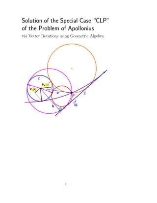
  • 6. 2 The Problem of Apollonius, and Its CLP Spe- cial Case The famous “Problem of Apollonius”, in plane geometry, is to construct all of circles that are tangent, simultaneously, to three given circles. In one variant of that problem, one of the circles has infinite radius (i.e., it’s a line). The Wikipedia article that’s current as of this writing has an extensive description of the problem’s history, and of methods that have been used to solve it. As described in that article, one of the methods reduces the “two circles and a line” variant to the so-called “Circle-Line-Point” (CLP) special case: Given a circle C, a line L, and a point P, construct the circles that are tangent to C and L, and pass through P. 2.1 Observations, and Potentially Useful Elements of the Problem From the figure presented in the statement of the problem, we can see that there are two types of solutions. That is, two types of circles that satisfy the stated conditions: • Circles that enclose C; • Circles that do not enclose C. We’ll begin by discussing circles that do not enclose C. Most of our obser- vations about that type will also apply, with little modification, to circles that do enclose C. Based upon our experience in solving other “construction problems in- volving tangency, a reasonable choice of elements for capturing the geometric 6
  • 7. content of the problem is as shown below: • Use the center point of the given circle as the origin; • Capture the perpendicular distance from c1’s center to the given line in the vector h; • Express the direction of the given line as ±ˆhi. • Label the solution circle’s radius and its points of tangency with C and L as shown below: In deriving our solution, we’ll use the same symbol —for example, t —to denote both a point and the vector to that point from the origin. We’ll rely upon context to tell the reader whether the symbol is being used to refer to the point, or to the vector. Now, we’ll express key features of the problem in terms of the elements that we’ve chosen. First, we know that we can write the vector s as s = h + λˆhi, where λ is some scalar. We also know that the points of tangency t and s are equidistant (by r2) from the center point of the solution circle. Combining those observations, we can equate two expressions for the vector s: s = (r1 + r2)ˆt + r2 ˆh = h + λˆhi. (1) 7
  • 8. Examining that equation, we observe that we can obtain an expression for r2 in terms of known quantities by “dotting” both sides with ˆh: (r1 + r2)ˆt + r2 ˆh · ˆh = h + λˆhi · ˆh (r1 + r2)ˆt · ˆh + r2 ˆh · ˆh = h · ˆh + λ ˆhi · ˆh (r1 + r2)ˆt · ˆh + r2 = |h| + 0; ∴ r2 = |h| − r1 ˆt · ˆh 1 + ˆt · ˆh . (2) The denominator of the expression on the right-hand side might catch our attention now because one of our two expressions for the vector s, namely s = (r1 + r2)ˆt + r2 ˆh can be rewritten as s = r1 ˆt + r2 ˆt + ˆh . That fact becomes useful (at least potentially) when we recognize that ˆt + ˆh 2 = 2 1 + ˆt · ˆh . Therefore, if we wish, we can rewrite Eq. (10) as r2 = 2    |h| − r1 ˆt · ˆh ˆt + ˆh 2    . Those results indicate that we should be alert to opportunities to simplify expressions via appropriate substitutions invoving ˆt + ˆh and 1 + ˆh · ˆt As a final observation, we note that when a circle is tangent to other objects, there will be many angles that are equal to each other. For example, the angles whose measures are given as θ in the following diagram: We’ve seen in Smith J A 2016 that GA expressions for rotations involving angles like the two θ’s often capture geometric content in convenient ways. 8
  • 9. 2.2 Identifying the Solution Circles that Don’t Enclose C Many of the ideas that we’ll employ here will also be used when we treat solution circles that do enclose C. 2.2.1 Formulating a Strategy Now, let’s combine our observations about the problem in a way that might lead us to a solution. Our previous experiences in solving problems via vector rotations suggest that we should equate two expressions for the rotation eθi : t − p |t − p| s − p |s − p| = t − s |t − s| −ˆhi = s − t |s − t| ˆhi . (3) We’ve seen elsewhere that we will probably want to transform that equation into one in which some product of vectors involving our unknowns t and s is equal either to a pure scalar, or a pure bivector. By doing so, we may find some way of identifying either t or s. We’ll keep in mind that although Eq. (3) has two unknowns (the vectors t and s), our expression for r2 (Eq. (10)) enables us to write the vector s in terms of the vector ˆt. Therefore, our strategy is to • Equate two expressions, in terms of the unknown vectors t and s, for the rotation eθi ; • Transform that equation into one in which on side is either a pure scalar or a pure bivector; • Watch for opportunities to simplify equations by substituting for r2; and • Solve for our unknowns. 2.2.2 Transforming and Solving the Equations that Resulted from Our Observations and Strategizing For convenience, we’ll present our earlier figure again: 9
  • 10. By examining that figure, we identified and equated two expressions for the rotation eθi , thereby obtaining Eq. (3): t − p |t − p| s − p |s − p| = s − t |s − t| ˆhi . We noted that we might wish at some point to make the substitution s = [r1 + r2]ˆt + r2 ˆh = r1 + |h| − r1 ˆt · ˆh 1 + ˆt · ˆh ˆt + |h| − r1 ˆt · ˆh 1 + ˆt · ˆh ˆh. (4) We also noted that we’ll want to transform Eq. (3) into one in which one side is either a pure scalar or a pure bivector. We should probably do that transformation before making the substitution for s. One way to effect the transformation is by left-multiplying both sides of Eq. (3) by s − t, then by ˆh, and then rearranging the result to obtain ˆh [s − t] [t − p] [s − p] = |s − t| |t − p| |s − p| i (5) This is the equation that we sought to obtain, so that we could now write ˆh [s − t] [t − p] [s − p] 0 = 0. (6) Next, we need to expand the products on the left-hand side, but we’ll want to examine the benefits of making a substitution for s first. We still won’t, as yet, write s in terms of ˆt. In hopes of keeping our equations simple enough for us to identify useful simplifications easily at this early stage, we’ll make the substitution s = (r1 + r2)ˆt + r2 ˆh, rather than making the additional substitution (Eq. (10)) for r2. Now, we can see that s − t = r2 ˆt + ˆh . Using this result, and t = r1 ˆt, Eq. (6) becomes ˆh r2 ˆt + ˆh r1 ˆt − p (r1 + r2)ˆt + r2 ˆh − p 0 = 0. 10
  • 11. Now here is where I caused myself a great deal of unnecessary work in previous versions of the solution by plunging in and expanding the product that’s inside the 0 without examining it carefully. Look carefully at the last factor in that product. Do you see that we can rearrange it to give the following? ˆh r2 ˆt + ˆh r1 ˆt − p r2 ˆt + ˆh + r1 ˆt − p After rearrangement 0 = 0. That result is interesting, but is it truly useful to us? To answer that question, let’s consider different ways in which we might expand the product, then find its scalar part. If we effect the multiplications in order, from left to right, we’re likely to end up with a confusing mess. However, what if we multiply the last three factors together? Those three factors, together, compose a product of the form ab [a + b]: r2 ˆt + ˆh a r1 ˆt − p b   r2 ˆt + ˆh a + r1 ˆt − p b    . The expansion of ab [a + b] is ab [a + b] = aba + b2 a = 2 (a · b) a − a2 b + b2 a (among other possibilites). That expansion evaluates to a vector, of course. Having obtained the cor- responding expansion of the product r2 ˆt + ˆh r1 ˆt − p r2 ˆt + ˆh + r1 ˆt − p , we’d then “dot” the result with ˆh to obtain ˆh r2 ˆt + ˆh r1 ˆt − p r2 ˆt + ˆh + r1 ˆt − p 0. We know, from the solutions to Problem 6 in Smith J A 2016 , that such a ma- neuver can work out quite favorably. So, let’s try it. Expanding r2 ˆt + ˆh r1 ˆt − p r2 ˆt + ˆh + r1 ˆt − p according to the identity ab [a + b] = 2 (a · b) a − a2 b + b2 a, we obtain, initially, 2 r2 2 ˆt + ˆh · r1 ˆt − p ˆt + ˆh − r2 2 ˆt + ˆh 2 r1 ˆt − p + r2 r1 ˆt − p 2 ˆt + ˆh When we’ve completed our expansion and dotted it with ˆh, we’ll set the result to zero, so let’s divide out the common factor r2 now: 2 r2 ˆt + ˆh · r1 ˆt − p ˆt + ˆh − r2 ˆt + ˆh 2 r1 ˆt − p + r1 ˆt − p 2 ˆt + ˆh Recalling that ˆt + ˆh 2 = 2 1 + ˆh · ˆt , the preceding becomes 2 r2 ˆt + ˆh · r1 ˆt − p ˆt + ˆh − 2r2 1 + ˆh · ˆt r1 ˆt − p + r1 ˆt − p 2 ˆt + ˆh . This is the form that we’ll dot with ˆh. Having done so, the factor ˆt+ ˆh becomes 1 + ˆh · ˆt. Then, as planned, we set the resulting expression equal to zero: 2 r2 ˆt + ˆh · r1 ˆt − p 1 + ˆh · ˆt − 2r2 1 + ˆh · ˆt r1 ˆh · ˆt − ˆh · p + r1 ˆt − p 2 1 + ˆh · ˆt = 0. 11
  • 12. Next, we’ll rearrange that equation to take advantage of the relation r2 = |h| − r1 ˆh · ˆt 1 + ˆh · ˆt (see Eq. (10)). We’ll show the steps in some detail: 2 r2 ˆt + ˆh · r1 ˆt − p 1 + ˆh · ˆt − 2r2 1 + ˆh · ˆt r1 ˆh · ˆt − ˆh · p + r1 ˆt − p 2 1 + ˆh · ˆt = 0. 2r2 1 + ˆh · ˆt ˆt + ˆh · r1 ˆt − p − r1 ˆh · ˆt + ˆh · p + r1 ˆt − p 2 1 + ˆh · ˆt = 0 2 |h| − r1 ˆh · ˆt 1 + ˆh · ˆt 1 + ˆh · ˆt ˆt + ˆh · r1 ˆt − p − r1 ˆh · ˆt + ˆh · p + r1 ˆt − p 2 1 + ˆh · ˆt = 0 2 |h| − r1 ˆh · ˆt ˆt + ˆh · r1 ˆt − p − r1 ˆh · ˆt + ˆh · p + r1 ˆt − p 2 1 + ˆh · ˆt = 0 2 |h| − r1 ˆh · ˆt r1 − p · ˆt + r1 ˆh · ˆt − ˆh · p − r1 ˆh · ˆt + ˆh · p + r1 ˆt − p 2 1 + ˆh · ˆt = 0 2 |h| − r1 ˆh · ˆt r1 − p · ˆt + r1 ˆt − p 2 1 + ˆh · ˆt = 0. Now that the dust has settled from the r2 substitution, we’ll expand r1 ˆt − p 2 , then simplify further: 2 |h| − r1 ˆh · ˆt r1 − p · ˆt + r1 2 − 2r1p · ˆt + p2 1 + ˆh · ˆt = 0 −2r1 2 + 2r1p · ˆt + r1 2 − 2r1 ˆt · p + p2 ˆh · ˆt − 2 |h| p · ˆt + 2 |h| r1 + r1 2 − 2r1p · ˆt + p2 = 0 p2 − r1 2 ˆh · ˆt − 2 (r1 + |h|) p · ˆt + r1 2 + p2 + 2 |h| r1 = 0. We saw equations like this last one many times in Smith J A 2016. There, we learned to solve those equations by grouping the dot products that involve t into a dot product of t with a linear combination of known vectors: 2 (r1 + |h|) p − p2 − r1 2 ˆh A linear combination of ˆh and p ·ˆt = 2 |h| r1 + r1 2 + p2 . (7) The geometric interpretation of Eq. (7) is that 2 |h| r1 +r1 2 +p2 is the pro- jection of the vector 2 (r1 + |h|) p− p2 − r1 2 ˆh upon ˆt. Because we want to find t, and know 2 (r1 + |h|) p − p2 − r1 2 ˆh, we’ll transform Eq. (7) into a version that tells us the projection of the vector t upon 2 (r1 + |h|) p − p2 − r1 2 ˆh. First, just for convenience, we’ll multiply both sides of Eq. (7) by r1 |h|: 2 r1 |h| + h2 p − p2 − r1 2 h · t = 2h2 r1 2 + r1 |h| r1 2 + p2 . Next, we’ll use the symbol “w” for the vector 2 r1 |h| + h2 p − p2 − r1 2 h , and write w · t = 2h2 r1 2 + r1 |h| r1 2 + p2 . Finally, because P w (t), the projection of the vector t upon w is (t · ˆw) ˆw, we have P w (t) = 2h2 r1 2 + r1 |h| r1 2 + p2 |w| ˆw. (8) 12
  • 13. As we learned in Smith J A 2016, Eq. (8) tells us that Eq (7) has two solutions. That is, there are two circles that are tangent to L and pass through the point P, and are also tangent to C without enclosing it: Having identified P w (t), the points of tangency with C and L can be determined using methods shown in Smith J A 2016, as can the equations for the corresponding solution circles. To round off our treatment of solution circles that don’t enclose C, we should note that we derived our solution starting from equations that express the relationship between C, L, P, and the smaller of the two solution circles. You may have noticed that the larger solution circle does not bear quite the same relationship to L, P, and C as the smaller one. To understand in what way those relationships differ, let’s examine the following figure. 13
  • 14. By equating two expressions for the rotation eψi , we’d find that s − p |s − p| t − p |t − p| = ˆhi t − s |t − s| . Compare that result to the corresponding equation for the smaller of the solution circles: t − p |t − p| s − p |s − p| = s − t |s − t| ˆhi . We followed up on that equation by transforming it into one in which ˆh was at one end of the product on the left-hand side. The result was Eq. (5): ˆh [s − t] [t − p] [s − p] = |s − t| |t − p| |s − p| i. We saw the advantages of that arrangement when we proceeded to solve for t. All we had to do in order to procure that arrangement was to left-multiply both sides of the equation t − p |t − p| s − p |s − p| = s − t |s − t| ˆhi by s − t, and then by ˆh. To procure a similar arrangement starting from the equation that we wrote for the larger circle, using the angle ψ , s − p |s − p| t − p |t − p| = ˆhi t − s |t − s| , we could left-multiply both sides of the equation by ˆh, then right-multiply by s − t, giving ˆh [s − p] [t − p] [t − s] = |s − p| |t − p| |t − s| i. Using the same ideas and transformations as for the smaller circle, we’d then transform the product [s − p] [t − p] [t − s] into r2 ˆt + ˆh + r1 ˆt − p r1 ˆt − p r2 ˆt + ˆh . By comparison, the product that we obtained for the smaller circle was r2 ˆt + ˆh r1 ˆt − p r2 ˆt + ˆh + r1 ˆt − p . In both cases, the products that result from the expansion have the forms ˆt + ˆh r1 ˆt − p ˆt + ˆh and r1 ˆt − p 2 ˆt + ˆh , so the same simplifications work in both, and give the same results when the result is finally dotted with ˆh and set to zero. The above having been said, let’s look at another way of obtaining an equa- tion, for the larger circle, that has the same form as Eq. (5). For convenience, we’ll present the figure for the larger circle again: 14
  • 15. Instead of beginning by equating two expressions for the rotation eψi , we’ll equate two expressions for e−ψi : t − p |t − p| s − p |s − p| = t − s |t − s| ˆhi . After left-multiplying both sides by t−s, then by ˆh, and rearranging, the result would be identical to Eq. (5), except for the algebraic sign of the right-had side, which —because it’s a bivector—would drop out when we took the scalar part of both sides. However, the difference in the sign of that bivector captures the geometric nature of the difference between the relationships of the large and small circles to L, P, and C. That difference in sign is also reflected in the positions, with respect to the vector w, of the solution circles’ points of tangency t: 15
  • 16. 2.3 Identifying the Solution Circles that Enclose C These solution circles can be found by modifying, slightly, the ideas that we used for finding solution circles that don’t enclose C. Here, too, we’ll want to express the radius r3 of the solution circle in terms of the vector t. Examining the next figure, we see that s = (r1 − r3)ˆt+r3 ˆh, and also that s = h+λˆhi. By equating those two expressions, dotting both sides with ˆh, and then solving for r3, we find that r3 = |h| − r1 ˆt · ˆh 1 − ˆt · ˆh . As was the case when we found solution circles that didn’t enclose C, we’ll want to equate expressions for two rotations that involve the unknown points of tangency t and s. For example, through the angles labeled φ, below: t − p |t − p| s − p |s − p| = t − s |t − s| −ˆhi = s − t |s − t| ˆhi , 16
  • 17. Left-multiplying that result by s − t, and then by ˆh, ˆh [s − t] [t − p] [s − p] = |s − t| |t − p| |s − p| i ∴ ˆh [s − t] [t − p] [s − p] 0 = 0, which is identical to Eq. (6). To solve for t, we use exactly the same technique that we did when we identified the solution circles that don’t surround C, with r3 and 1 − ˆh · ˆt taking the place of r2 and 1 − ˆh · ˆt, respectively. The result is z · t = 2h2 r1 2 − r1 |h| r1 2 + p2 , where z = 2 h2 − r1 |h| p − p2 − r1 2 h . Thus, P z (t) = 2h2 r1 2 − r1 |h| r1 2 + p2 |z| ˆz. (9) Again, there are two solution circles of this type: 2.4 The Complete Solution, and Comments There are four solution circles: two that enclose C, and two that don’t: 17
  • 18. I confess that I don’t entirely care for the solution presented in this document. The need to identify r2, in order to eliminate it later, makes me suspect that I did not make good use of GA’s capabilities. A solution that uses reflections in addition to rotations is in preparation, and is arguably more efficient. 3 Literature Cited GeoGebra Worksheets and Related Videos (by title, in alphabetical order): ”Answering Two Common Objections to Geometric Algebra” GeoGebra worksheet: http://tube.geogebra.org/m/1565271 YouTube video: https://www.youtube.com/watch?v=oB0DZiF86Ns. ”Geometric Algebra: Find unknown vector from two dot products” GeoGebra worksheet: http://tube.geogebra.org/material/simple/id/1481375 YouTube video: https://www.youtube.com/watch?v=2cqDVtHcCoE Books and articles (according to author, in alphabetical order): Gonz´alez Calvet R. 2001. Treatise of Plane Geometry through Geometric Algebra. 89.218.153.154:280/CDO/BOOKS/Matem/Calvet.Treatise.pdf. Retrieved 30 December 2015. Hestenes D. 1999. New Foundations for Classical Mechanics (Second Edition). Kluwer Academic Publishers, Dordrecht/Boston/London. 18
  • 19. Macdonald A. 2010. Linear and Geometric Algebra. CreateSpace Independent Publishing Platform, ASIN: B00HTJNRLY. Smith J. A. 2014. “Resoluciones de ’problemas de construcci´on’ geom´etricos por medio de la geometr´ıa cl´asica, y el ´Algebra Geom´etrica”, http://quelamatenotemate.webs.com/3%20soluciones %20construccion%20geom%20algebra%20Cliffod.xps 2016. “Rotations of Vectors via Geometric Algebra: Explanation, and Usage in Solving Classic Geometric “Construction” Problems” https://drive.google.com/file/d/0B2C4TqxB32RRdE5KejhQTzMtN3M/view?usp=sharing 4 APPENDIX: Improved Solutions We’ll show two ways of solving the problem; the second takes advantage of observations made during the first. As noted in the main text, the CLP limiting case reads, Given a circle C, a line L, and a point P, construct the circles that are tangent to C and L, and pass through P. Figure 1: The CLP Limiting Case of the Problem of Apollonius: Given a circle C, a line L, and a point P, construct the circles that are tangent to C and L, and pass through P. The problem has two types of solutions: • Circles that enclose C; • Circles that do not enclose C. 19
  • 20. There are two solution circles of each type. In this document, we’ll treat only those that do not enclose the given circle. 4.1 The First Solution Fig. 2 shows how we will capture the geometric content of the problem. An important improvement, compared to the solution technique presented in [?], is that we will use rotations with respect to the vector from the given point P to the still-unidentified center point (c2) of the solution circle. Figure 2: Elements used in the first solution of the CLP limiting case. In deriving our solution, we’ll use the same symbol —for example, t —to denote both a point and the vector to that point from the origin. We’ll rely upon context to tell the reader whether the symbol is being used to refer to the point, or to the vector. We’ll begin our solution by deriving an expression for r2 in terms of ˆt. We´ll do so by equating two independent expressions for s, then “dotting” both sides with ˆh, after which we’ll solve for r2: (r1 + r2)ˆt + r2 ˆh = h + λˆhi (r1 + r2)ˆt + r2 ˆh · ˆh = h + λˆhi · ˆh (r1 + r2)ˆt · ˆh + r2 ˆh · ˆh = h · ˆh + λ ˆhi · ˆh (r1 + r2)ˆt · ˆh + r2 = h + 0; ∴ r2 = h − r1 ˆt · ˆh 1 + ˆt · ˆh , and r1 + r2 = h + r1 1 + ˆt · ˆh . (10) Next, we equate two expressions for the rotation ei2φ : t − p t − p c2 − p c2 − p =eiφ t − p t − p c2 − p c2 − p =eiφ = −ˆt c2 − p c2 − p =ei2φ , 20
  • 21. from which [t − p] [c2 − p] [t − p] ˆt = some scalar, ∴ [t − p] [c2 − p] [t − p] ˆt 2 = 0. (11) Using the identity ab ≡ 2a ∧ b + ba, we rewrite 11 as (2 [t − p] ∧ [c2 − p] + [c2 − p] [t − p]) [t − p] ˆt 2 = 0, (2 [t − p] ∧ [c2 − p]) [t − p] ˆt + [t − p] 2 [c2 − p] ˆt 2 = 0, and (2 [t − p] ∧ [c2 − p]) [t − p] ˆt 2 + [t − p] 2 [c2 − p] ˆt 2 = 0. (12) Now, we note that (2 [t − p] ∧ [c2 − p]) [t − p] ˆt 2 = 2 ([t − p] ∧ [c2 − p]) [t − p] · ˆt , and [t − p] 2 [c2 − p] ˆt 2 = [t − p] 2 [c2 − p] ∧ ˆt . Note how the factor p ∧ ˆt canceled out in Eq. (13). That cancellation suggests an improvement that we’ll see in our second solution of the CLP case. Because t = r1 ˆt and c2 = (r1 + r2)ˆt, t ∧ c2 = 0. We can expand [t − p] 2 as r1 2 − 2p · t + p2 . Using all of these ideas, (12) becomes (after simplification) 2r2 r1 − p · ˆt p ∧ ˆt + r1 2 − 2p · t + p2 p ∧ ˆt = 0. (13) For p ∧ ˆt = 0, that equation becomes 2r2 r1 − p · ˆt + r1 2 − 2p · t + p2 = 0. Substituting the expression that we derived for r2 in (10), then expanding and simplifying, 2 ( h + r1) p · ˆt − p2 − r1 2 ˆh · ˆt = 2 h r1 + r1 2 + p2 . Finally, we rearrange that result and multiply both sides by r1 h , giving the equation that we derived in [?]: 2 r1 h + h2 p − p2 − r1 2 h · t = 2h2 r1 2 + r1 h r1 2 + p2 . (14) 4.2 The Second Solution: Learning From and Building Upon the First In Eq. (13), we saw how the factor p∧ˆt canceled out. That cancellation suggests that we might solve the problem more efficiently by expressing rotations with respect to the unknown vector ˆt, rather than to a vector from P to c2 (Fig. 3). For this new choice of vectors, our equation relating two expressions for the rotation ei2φ is: ˆt p − t p − t =eiφ ˆt p − t p − t =eiφ = ˆt p − c2 p − c2 =ei2φ , 21
  • 22. Figure 3: Elements used in the second solution of the CLP Limiting Case: rotations are now expressed with respect to the unknown vector ˆt, rather than to a vector from P to c2. from which [p − t] ˆt [p − t] [p − c2] = some scalar, ∴ [p − t] ˆt [p − t] [p − c2] 2 = 0. (15) Using the identity ab ≡ 2a ∧ b + ba, we rewrite 15 as 2 [p − t] ∧ ˆt + ˆt [p − t] [p − t] [p − c2] 2 = 0, and 2 [p − t] ∧ ˆt [p − t] [p − c2] 2 + [p − t] 2 ˆt [p − c2] 2 = 0. (16) Now, we note that 2 [p − t] ∧ ˆt [p − t] [p − c2] 2 = 2 [p − t] ∧ ˆt [p − t] · [p − c2] , and [p − t] 2 ˆt [p − c2] 2 = [p − t] 2 ˆt ∧ [p − c2] . Because t = r1 ˆt and c2 = (r1 + r2)ˆt, t ∧ c2 = 0. We can expand [p − t] 2 as p2 − 2p · t + r1 2 . Using all of these ideas, (16) becomes (after simplification) 2 ([p − t] · [p − c2]) p ∧ t − p2 − 2p · t + r1 2 p ∧ t = 0. For p ∧ ˆt = 0, that equation becomes, after expanding [p − t] · [p − c2] and further simplifications, p2 − r1 2 − 2p · c2 + 2t · c2 = 0. Now, recalling that c2 = (r1 + r2)ˆt, we substitute the expression that we derived for r1 + r2 in (10), then expand and simplify to obtain (14). This solution process has been a bit shorter than the first because (16) was so easy to simplify. 22