SlideShare a Scribd company logo
1 of 64
M210 Songyue.pages
__MACOSX/._M210 Songyue.pages
M210-S16-class-5.pdf
M 210 More drawing in LATEX February 23, 2016
Arcs
An arc of radius r from point (p,q) with initial angle ϕ (phi) and
final angle ψ (psi) is drawn in
TikZ by the code
LATEXdraw (p,q) arc (phi:psi:r);
Note that TikZ does not require the center (a,b), which is often
easier to determine that the arc’s
initial point. Polar coordinates (relative to the arc’s center) can
be used to express the initial point
in terms of the arc’s center.
(a,b)
(p,q)
ϕ
ψ
r
p = a + r cosϕ
q = b + r sinϕ
In tikzpicture environment enter
draw ({a+r*cos(phi)},{b+r*sin(phi)}) arc (phi:psi:r);
for the specific values of a, b, r, ϕ (phi) and ψ (psi).
LATEX
According to the TikZ’s manual, by default arcs are drawn in
positive (counter-clockwise) direction,
assuming initial angle ϕ to be smaller than ψ. However, I have
been able to draw arcs in negative
(clockwise) direction by choosing an initial angle larger than
final angle.
Precise Label Positioning
The relative positions above, below, left, right, above left,
above right, below left, and
below right, provide positioning relative to the node (indicated
by the dot) as illustrated in the
following figures.
below
above
left right
above left
below left
above right
below right
While it is possible to adjust the separation between label and
node, it is not that easy to adjust
the angle (the above provide label placement only for angles in
multiples of 45◦). The following will
work to place the label (that is its center) at the the indicated
position: precise distance s at relative
angle θ from the position of the node.
node
lab
el
s
node coordinates (nx,ny)
label coordinates (lx, ly)
θ
To place label at the above mentioned position use the code
(where θ is theta degrees):
M 210 — February 23, 2016 page 44
LATEXdraw ({nx + s*cos(theta)}, {ny + s*sin(theta)}) node
{label};
To rotate the label as in the above illustration, use code:
LATEXdraw ({nx + s*cos(theta)}, {ny + s*sin(theta)}) node
{rotatebox{theta}{label}};
Special Triangles
In trigonometry the triangles with degrees 45-45-90 and 30-60-
90 provide exact values for the trigono-
metric functions. It is quite easy to obtain the exact values of
angles of 15 and 75 degrees from those
of 30 degrees by half- and double-angle formulas and other
trigonometric identities, however, these
values can also be obtained from the following figure
containing an equilateral triangle in a square
with sides equal to 2.
1
The Regular Pentagon. Use trigonometric functions to draw a
regular pentagon with its lower
side along the line segment from (−1,0) to (1,0). Start by
drawing this line segment.
LATEXbegin{center}
begin{tikzpicture}[scale=2]
draw[line width=1.2pt] (-1,0) -- (1,0);
end{tikzpicture}
end{center}
Extend the line segment on both sides by adding the following
code.
LATEXdraw[line width=1.2pt] (1,0) --
({1+2*cos(72)},{2*sin(72)});
draw[line width=1.2pt] (-1,0) -- ({-1-2*cos(72)},{2*sin(72)});
Close the top of the pentagon, using angles denoted in the
desired figure on the following page, by
adding the following code.
LATEXdraw[line width=1.2pt]
({1+2*cos(72)},{2*sin(72)})--(0,{2*sin(72)+2*sin(36)})--({-1-
2*cos(72)},{2*sin(72)});
Of course we can shorten the code by placing it all in one string
using --cycle to close the pentagon’s
path.
M 210 — February 23, 2016 page 45
Now add the following lines to provide a coordinate system.
LATEXdraw[gray] (-2,0)--(2,0);
draw[gray] (0,-.25)--(0,3.35);
Add the second gray horizontal line.
Color and label the indicated angles. The yellow angle with the
x-axis was obtained by the following
code.
LATEXdraw[fill=yellow!50] (1,0)--(1.55,0) arc (0:72:0.55) --
cycle;
Use this as an example to draw the other angles.
108◦
72◦
72◦
36◦
1
1/2 cos(72◦)
cos(36◦)
From the figure we see
cos(36◦) =
1
2
+ cos(72◦).
Using the double angle formula for the cosine we have
cos(36◦) =
1
2
+ 2 cos2(36◦) − 1,
which can be rewritten as
4 cos2(36◦) − 2 cos(36◦) − 1 = 0.
Because cos(36◦) > 0, with the help of the quadratic formula we
conclude
cos(36◦) =
2 +
√
4 − 4(4)(−1)
8
=
2 +
√
20
8
=
√
5 + 1
4
.
It follows that
cos(72◦) =
√
5 − 1
4
.
See TikZercise 3 for an alternative derivation.
Construction Regular Pentagon.
Draw a unit circle, and let A and B be the points (0,1) and
(−1,0), respectively.
M 210 — February 23, 2016 page 46
B
O
A
Let C be the midpoint of OB. Then by the Pythagorean Theorem
we have
AC2 = (1/2)2 + 12 = 5/4 =⇒ AC =
1
2
√
5.
B
O
A
C
Use AC as length for a pentagon, constructed as indicated in the
following figure.
M 210 — February 23, 2016 page 47
B
O
A
C
D
EF
Homework 4
TikZercises. Draw the following in a LATEX document using
TikZ:
1. Draw the following proof of the Pythagorean Theorem.
a b
c
c
c
c
b a
b
a
a
b
a
a
a
b
b
b
M 210 — February 23, 2016 page 48
2. Draw the figure from page 44 with all angles labelled, and
use the figure to find the exact
values of cos, sin and tan at angles 15◦ and 75◦.
3. Draw a right-angled triangle with angles 72◦ and 18◦ whose
side adjacent
angle 72◦ has length 1 as shown in the adjacent figure.
To determine the exact value of hypotenuse x, first put two such
triangles
together as indicated in the following figure. Next, extend the
above tri-
angles’ base, mark a point E length x to the left of A along the
base and
complete a larger triangle BDE as shown in the following
figure.
72◦
18◦
x
1A
B
C
72◦ 72◦
18◦ 18◦
x
1 1x A
B
C
DE
Answer the following questions in your LATEX document:
(a) Find the missing angles ∠ AEB and ∠ ABE.
(b) Show that triangles DBE and ADB are similar.
(c) Using the similarity of triangles DBE and ADB, set up an
equation for x and solve this
equation.
(d) Find the missing sides and angles in the following two
special right triangles, then draw
them showing all sides and angles.
M 210 — February 23, 2016 page 49
72◦
18◦
1A C
B
E C
B
4. Draw the following figure with missing angles (indicated by
arcs) and line segments filled in,
and use this information to find identities for cos(α + β) and
sin(α + β).
[Use optional argument rotate=ang in draw for appropriate
angle ang (in degrees) to rotate
the line segments to denote a right angle.]
α
β
1
M 210 — February 23, 2016 page 50
5. On the legs of angle ∠ ABC points P , Q, R and S are so that
all five blue segments are equal
(BP = PS = SR = RQ = BQ). Draw this figure and show that
∠ ABC = 36◦.
C
AB
R
S
P
Q
6. The following figure
1/2
1/4
1/8
1/16
1/32
1/64
1/128
1
256
shows that
1
2
+
1
4
+
1
8
+
1
16
+
1
32
+
1
64
+
1
128
+
1
256
+ · · · = 1.
Using summation notation, the above states that
∞
∑
k=1
1
2k
= 1.
M 210 — February 23, 2016 page 51
7. Draw the following figure and typeset the derivation of the
Law of Cosines following the figure.
θ
a c
b
acosθ b − acosθ
a
si
n
θ
The Pythagorean Theorem applied to the right-angled triangle
results in
c2 = (asinθ)2 + (b − acosθ)2
= a2 sin2 θ + b2 + a2 cos2 θ − 2ab cosθ
= a2(cos2 θ + sin2 θ) + b2 − 2ab cosθ
= a2 + b2 − 2ab cosθ.
8. Draw the following figure.
θ
θ
1
cos
θ
sin
θ
cos2 θ
sin2 θ
θ
co
s
θ
sin
θ
co
s
θ
sin
θ
Behold:
cos 2θ = cos2 θ − sin2 θ,
sin 2θ = 2 cosθ sinθ.
9. Draw the following figure, and typeset the conclusions.
M 210 — February 23, 2016 page 52
A BC
P
θ
θ
1
2θ
Q
cos 2θ
sin 2θ
cos
θ
cos
θ
Considering right △APQ, it follows from the figure that
sinθ =
sin 2θ
2 cosθ
,
cosθ =
1 + cos 2θ
2 cosθ
,
from which the identities
sin 2θ = 2 cosθ sinθ,
cos 2θ = 2 cos2 θ − 1.
follow easily.
Submit Homework 4 by 3:00pm on Tuesday, March 1, to
Moodle.
Please put course, your last name, and homework number in the
name of the file you submit (using
a file name like M210-HW4-name).
__MACOSX/._M210-S16-class-5.pdf
M210-S16-class-7.pdf
M 210 Introduction to Mathematica March 8, 2016
Creator of Mathematica
British-born Stephen Wolfram received a Ph.D. in particle
physics
from the California Institute of Technology at age 20. In 1986
Wolfram
founded the Center for Complex Systems Research at the
University
of Illinois at Urbana-Champaign and started to develop the
computer
algebra system Mathematica, which was first released in 1988,
when
he left academia. In 1987 he co-founded a company called
Wolfram
Research which continues to develop and market the program.
Stephen Wolfram
Formatting
Stylesheet from Format from the menu contains several
stylesheets that can be used to change the
appearance of a Mathematica Notebook. Title and sections
header can be selected from Style from
the menu. Clicking the plus (+) symbols following an output
cell will bring up a window from which
one can select Plain text or Other style text to include in the
Notebook.
Notational Conventions
During a Mathematica session input cells and output cells are
labelled In[1], Out[1], In[2], Out[2],
In[3], Out[3], etc. Input cells are evaluated by either the enter
key or the shift-return key.
Built-in Mathematica commands and functions always begin
with a capital letter. It is good practice
to use lowercase letters for user defined objects. Function
arguments are always enclosed by square
brackets [ ]. Parentheses ( ) are used to group objects together,
and to establish priority of opera-
tions. Standard arithmetic operations are +, -, *, /, and ^. A
space is interpreted as multiplication:
xy is not the same as x*y, but the latter is the same as x y.
Variable names cannot start with
numbers, but otherwise numbers can occur, for example as
subscripts. Greek letters can be entered
and used, and something like ∆x can be a single variable.
Comments are delimited by (* and *).
The symbol % refers to the previous output, %% to the second-
previous output, etc. It is also
possible to refer to the output following Out[n] by using Out[n]
or simply by %n. Output can be
given in TraditionalForm, which is an attempt to match
traditional mathematical notation. While
it is possible to use TraditionalForm also for input, it is better
to use StandardForm, which is the
default for both input and output.
Calculator
When he was ten years old, the calculating prodigy Truman
Henry Safford (1836–1901) of Royalton,
Vermont, was once asked to square, in his head, the number
365,365,365,365,365,365. His church
leader reports, “He flew around the room like a top, pulled his
pantaloons over the tops of his boots,
bit his hands, rolled his eyes in their sockets, sometimes smiling
and talking, and then seeming to be in
agony, until in not more than a minute said he,
133,491,850,208,566,925,016,658,299,941,583,225”[1].
• Verify Safford’s answer using Mathematica.
Mathematical Constants
Mathematica contains several mathematical constants such as Pi
for π, E for Euler’s number e, I
for the imaginary number i =
√
−1, and GoldenRatio for the golden ratio.
M 210 — March 8, 2016 page 63
Some of these constants can be displayed similarly to the usual
notation, such as π, e, and i, by
making use of the escape key Esc , as follows:
Traditional form Key sequence
π Esc p Esc
e Esc ee Esc
i Esc ii Esc
Likewise, superscripts and subscripts can be obtained
combining the control key with ^ and -.
Traditional form Key sequence
x2 x Ctrl 6 2 >
x1 x Ctrl - 1 >
• Use Mathematica to evaluate eπi (make sure to leave space
between the two symbols in the
exponent; the answer should be −1).
The letters N and D cannot be used as names for user defined
objects; they are built-in commands:
the first for numerical approximation, the second for
differentiation. Mathematica displays only six
decimals by default when the numerical approximation N is
applied. To get m digits of expr enter
N[expr,m].
• Have Mathematica calculate 100 digits of π and of e.
• Which is larger πe or eπ? (The first computes to less than 23,
the second to a number larger
than 23.)
The StandardForm of Infinity can also be obtained using the
escape key. Greek letters can be
input using the escape key. The following table contains
keyboards shortcuts for some common
symbols.
Key sequence Result Full Name
Esc a Esc α [Alpha]
Esc D Esc ∆ [CapitalDelta]
Esc inf Esc ∞ [Infinity]
Esc e Esc ǫ [Epsilon]
Esc ce Esc ε [CurlyEpsilon]
Esc deg Esc ◦ [Degree]
Esc -> Esc → [Rule]
Esc => Esc ⇒ [Implies]
The golden ratio is often denoted by the Greek letter phi in
honor of the Greek sculptor Phidias (ca
480 BC–430 BC).
• Use the letter ϕ for the golden ratio (can be input in
Mathematica as Esc cphi Esc ), then
simplify ϕ2 − ϕ.
In[1]:= ϕ = GoldenRatio
In[2]:= Simplify[ϕ2 − ϕ]
In[3]:= Solve[x^2 - x == 1]
• What can you conclude about ϕ?
The golden ratio is the largest root of the above equation, which
is the number
ϕ =
√
5 + 1
2
.
This is the constant GoldenRatio in Mathematica (the other root
of the above equation is the
reciprocal of this constant).
M 210 — March 8, 2016 page 64
Symbolic Calculator
If a variable var has been assigned a value this can be undone
by using Clear[var] or, equivalently,
inputting var =.. Once a variable has been assigned a value,
Mathematica will substitute that value
in all calculations of the session. For example, suppose we have
calculated an expression to be
5 − 3x + x3, and now wish to evaluate this at x = 2. Far easier
than to assign value 2 to variable x,
then evaluate the expression, and finally clearing x, as indicated
in the following sequence of code
Out[1]= 5 - 3 x + x^3
In[2]:= x=2
Out[2]= 2
In[3]:= %%
Out[3]= 7
In[4]:= x=.
would be to substitute the value of x into the given expression
using /. followed by a value assignment
to x using a right arrow as follows.
Out[1]= 5 - 3 x + x^3
In[2]:= % /. x → 2
Out[2]= 7
Substitution using /. makes it unnecessary to unclear the
variable.
Lists
Mathematica uses braces { and } for ordered lists, with the
elements contained in the lists separated
by commas.
If L denotes a list, then L[[k ]] gives its kth entry. The double
square brackets are entered using the
escape key: Esc [[ Esc gives [[ and ]] is obtained similarly. Note
that the escaped double square
brackets only serve an esthetic purpose (visually showing the
components as functions of the list);
using plain double brackets [[ and ]] will work as well (and
saves key strokes).
In[1]:= L = {1, 8, 28, 56, 70, 56, 28, 8, 1}
Out[1]= {1, 8, 28, 56, 70, 56, 28, 8, 1}
In[2]:= L[[4]]
Out[2]= 56
The command Table can be used to create lists generated by
formulas. For example
In[3]:= T = Table[i^2, {i, 10}]
Out[3]= {1, 4, 9, 16, 25, 36, 49, 64, 81, 100}
These lists can be manipulated with the various arithmetic
operators.
• Investigate the result of adding and multiplying these lists,
and squaring each of them.
Lists can be plotted using the ListPlot command:
In[4]:= ListPlot[L]
The built-in function Prime gives the prime numbers in order.
We can generate a list of the first
1000 prime numbers:
In[5]:= Table[Prime[i], {i, 1000}]
M 210 — March 8, 2016 page 65
Sums and Series
Evaluate some partial sums of the series
∑∞
n=1 1/n
2.
In[1]:= Sum[1/n2, {n, 1, 10}]
In[2]:= Sum[1/n2, {n, 1, ∞}]
Integral
Integrals are evaluated similarly to sums. Evaluate the integral
∫ 1
0
x4(1 − x)4
1 + x2
dx
by entering the following.
In[1]:= Integrate[x^4(1 - x)^4/(1 + x^2), {x, 0, 1}]
The answer is 22
7
− π. The above integral provides a means of estimating the error
in the approxi-
mation π ≈ 22
7
; see the next example.
Plotting
We can plot the function in the above integral as follows.
In[1]:= Plot[x^4(1 - x)^4/(1 + x^2), {x, 0, 1}]
Locate the maximum of the above function, by setting its
derivative equal to zero to find its critical
point. Use this to estimate the integral, and thus obtain a bound
for the exact answer of the integral
obtained earlier. Following are the first steps of the above
procedure.
In[2]:= D[x^4(1 - x)^4/(1 + x^2), x]
In[3]:= Solve[% == 0,x]
In[4]:= x^4 (1 - x)^4/(1 + x^2) /. %[[7]]
In[5]:= N[%]
The computed result of 0.00315543 gives an upperbound for the
integral
∫ 1
0
x4(1−x)4
1+x2
dx, and thus
an upperbound for the error in the approximation π ≈ 22
7
.
Functions
Functions are defined using delayed assignment := and
indicating variable by following them with
underscores.
In[1]:= f[x_]:=x^2
In[2]:= f[a+b+c] // Expand
Note that if Fcn is a function, expr // Fcn is short-hand for
Fcn[expr].
In[3]:= (f[x+h]-f[x])/h // Simplify
M 210 — March 8, 2016 page 66
Animation
Define the cycloid by
In[1]:= Cycloid[t_] := {t - Sin[t], 1 - Cos[t]}
This is a parametric curve that can be plotted using
ParametricPlot:
In[2]:= ParametricPlot[Cycloid[t], {t, 0, 2 Pi}]
The following creates a simple animation.
Animate[Graphics[{
{EdgeForm[{Black, Thick}], Yellow, Disk[{t, 1}]},
Line[{{-1, 0}, {7, 0}}],
{Thick, Line[{{t, 1}, Cycloid[t]}]},
Disk[Cycloid[t], .075]}],
{t, 0, 2 Pi}]
Immediate versus Delayed Assignment
An immediate assignment is made using =, while := is used for
a delayed assignment. If we set
variable x equal to 2 by using as input x=2, then variable x will
be replaced by the number 2. The
function Random with empty argument generates a random
number between 0 and 1.
In[1]:= x = Random[]
In[2]:= {x, x, x}
Compare the output generated by the above code with that of
In[3]:= y := Random[]
In[4]:= {y, y, y}
An Example of Simplification
Use Mathematica to simplify
(
√
6 −
√
2)(
√
3 +
√
2) − 2
√
(
√
6 −
√
2)(
√
3 +
√
2)
.
The command Simplify has little effect. We can use the
command FullSimplify, which simplifies
the given expression. Mathematica simplifies the expression to
an expression containing nested
radicals, which it does not simply any further. Help
Mathematica to see if the expression can be
further simplified to a number that involves
4
√
2 and its reciprocal. [Suggestion: consider the square
of 21/4 − 2−1/4.]
In[1]:= q=((Sqrt[6]-Sqrt[2])(Sqrt[3]+Sqrt[2])-2)/Sqrt[(Sqrt[6]-
Sqrt[2])(Sqrt[3]+Sqrt[2])]
In[2]:= Simplify[q]
In[3]:= FullSimplify[q]
M 210 — March 8, 2016 page 67
Using FullSimplify Mathematica arrives at the answer
√
6
√
2 − 8 (Mathematica displays this in
different order, use TraditionalForm[%] to see identical output
by Mathematica). Can this answer
possibly be simplified? Let’s use Mathematica to calculate the
square of
4
√
2−1/ 4
√
2. Using fractional
exponents we enter this in Mathematica as follows.
In[4]:= (2^(1/4)-2^(-1/4))^2 // Expand
The answer is reminiscent of the earlier output above. In fact,
let’s have Mathematica compare
the result of the last computation with the expression under the
square root of its answer to the
FullSimplify command:
In[5]:= %/(-8 + 6 Sqrt[2]) // Expand
Mathematica’s answer shows that twice the number
4
√
2 − 1/ 4
√
2 is
√
6
√
2 − 8, so that our origi-
nal expression (in Mathematica stored in variable q) would be
equal to 2(
4
√
2 − 1/ 4
√
2). Let’s use
Mathematica to verify this:
In[6]:= FullSimplify[q - 2(2^(1/4)-2^(-1/4))]
The calculation confirms that we have found a simplified
answer for the original fraction:
(
√
6 −
√
2)(
√
3 +
√
2) − 2
√
(
√
6 −
√
2)(
√
3 +
√
2)
= 2
(
4
√
2 − 1
4
√
2
)
.
Using the rules of exponents we can rewrite the right-hand side
of the above formula as
2 · 21/4 − 2 · 2−1/4 = 25/4 − 23/4.
Mathematica’s command FullSimplify can also be used to
confirm this result:
In[7]:= FullSimplify[q - (2^(5/4)-2^(3/4))]
We have the following pretty simplification:
(
√
6 −
√
2)(
√
3 +
√
2) − 2
√
(
√
6 −
√
2)(
√
3 +
√
2)
= 25/4 − 23/4.
This example shows that while a computer algebra system
(CAS) is very useful in simplifying
complicated expressions, it may be necessary to provide
intelligent coaching to get at expressions
the CAS may not directly supply.
Special Trigonometric Values
Use Mathematica to verify the following formula for the cosine
(arrived at by several applications of
double-angle formulas):
cos 4θ = 1 − 8 sin2 θ + 8 sin4 θ. (1)
Simplify[Cos[4 [Theta]] - 1 + 8 Sin[[Theta]]^2 - 8
Sin[[Theta]]^4]
Observing that 90◦ − 18◦ = 72◦ = 4(18◦), we easily see that
sin(18◦) = cos 4(18◦), so by (1)
x = sin(18◦) satisfies the equation
x = 1 − 8x2 + 8x4. (2)
Use Mathematica to solve (2), and deduce from Mathematica’s
answer the exact value of sin(18◦).
Verify your answer using Mathematica.
There are several ways to solve the above polynomial equation.
First it is easy to see that x = 1 is
a solution so that x − 1 is a factor of the polynomial 8x4 − 8x2
− x + 1, and we can divide to obtain
the quotient:
M 210 — March 8, 2016 page 68
(8x^4-8x^2-x+1)/(x-1) // Simplify
The quotient is 8x3 + 8x2 − 1. We can has Mathematica
evaluate this at −1/2 by entering:
8x^3+8x^2-1 /. x->-1/2
Since the result is 0 also x − (−1/2) = x + 1/2 is a factor, so also
2x + 1. Divide this out:
(8x^3+8x^2-1)/(2x+1) // Simplify
The resulting quotient is 4x2 +2x−1, and x = sin(18◦) is a
solution of the equation 4x2 +2x−1 = 0.
Using the quadratic formula we get x = −1±
√
5
4
. Because sin(18◦) > 0 we conclude that
sin(18◦) =
√
5 − 1
4
.
An alternative is to factor the given polynomial 8x4 − 8x2 − x +
1:
Factor[8x^3+8x^2-1]
Another alternative is to use Mathematica’s built-in solver:
Solve[8x^3+8x^2-1,x]
Using the subtraction formula for the sine and the exact values
for sin(15◦) and cos(15◦) it is now
easy to find an exact values for sin(3◦) and cos(3◦); see the first
homework problem on page 136.
Another Example of Simplification
Use Mathematica to show that
√
5(1 +
5
√
4) =
5
√
2 +
5
√
8 +
5
√
16 − 1.
We enter the expressions into variables a and b in Mathematica:
a=Sqrt[5(1+Surd[4,5])]
b=Surd[2,5]+Surd[8,5]+Surd[16,5]-1
We can have Mathematica numerically approximate each of
these quantities:
N[a]
N[b]
The above calculation does not establish the above formula (the
calculation merely shows that the
quantities are close to each other). To show the formula we
need to use algebra. The following
computes the square of quantity b:
b^2
Expand[%]
Since b is positive, validity of the formula is now established.
A Third Example of Simplification
Use Mathematica to simplify
3
√
2 +
√
5 +
3
√
2 −
√
5. The numbers a =
3
√
2 +
√
5 and b =
3
√
2 −
√
5
satisfy a3 = 2 +
√
5 and b3 = 2 −
√
5, so a3 + b3 = 4. Before we enter these into Mathematica, lets
do some algebra:
M 210 — March 8, 2016 page 69
Clear[a,b]
(a+b)^3 // Expand
/. a^3+b^3->4
Factor waht remains after subtracting 4:
Factor[%-4]
Now observe that ab is easily computed, because (2 +
√
5)(2 −
√
5) = −1. So x = a + b satisfies the
equation x3 = 4 − 3x, that is x3 + 3x − 4 = 0. The calculation
Solve[x^3+3x-4==0]
shows that this cubic equation has one real real root, thus
3
√
2 +
√
5 +
3
√
2 −
√
5 = 1, a result that
can also be obtained using Mathematica’s FullSimplify instead
of Simplify (which does not do
anything with this input).
Some Plotting Options
The AspectRatio is by default set to the reciprocal of the golden
ratio. Turning it to Automatic
will set the same aspect ratio along the x- and y-axis.
Test with the function y =
√
1 − x2, −1 ≤ x ≤ 1.
Compare
Plot[Sqrt[1-x^2], {x, -1, 1}]
and
Plot[Sqrt[1-x^2], {x, -1, 1}, AspectRatio -> Automatic]
A list of functions can be plotted together, for example
Plot[{Sin[x], Sin[2x]}, {x, 0, 2 Pi}]
It is possible to have the plot display labels when the cursor is
placed over one of the functions
graphed. This is done using the function Tooltip, which takes
two arguments: first the function,
and second the label, entered between quotation marks.
Example:
Plot[{Tooltip[Sin[x], "sin x"], Tooltip[Sin[2 x], "sin 2x"]}, {x,
0, 2 Pi}]
The above plot has the same appearance as the one before, but
see what happens when the cursor
is moved over one of the graphs.
We can change the color and thickness of the graph by using the
option PlotStyle, for example
PlotStyle->{Thickness[0.005], Red}. If there is a list of
functions, PlotStyle needs to be
assigned to a list.
Plot[{Sin[x], Sin[2x]}, {x, 0, 2 Pi},
PlotStyle -> {{Thickness[0.005], Red}, {Thickness[0.0075],
Blue}}]
We can add axes labels and ticks along the x-axis at π/2, π,
3π/2, 2π by adding AxesLabel and
Ticks options:
Plot[{Sin[x], Sin[2x]}, {x, 0, 2 Pi},
PlotStyle -> {{Thickness[0.005], Red}, {Thickness[0.0075],
Blue}}
AxesLabel -> {x, y}, Ticks -> {{Pi/2, Pi, 3 Pi/2, 2 Pi},
Automatic}]
M 210 — March 8, 2016 page 70
Note that Ticks is assigned a list of specification for the first
and second axis. In the above
example Automatic is chosen for the ticks along the second
axis. Another possibility is None, which
produces no ticks. Note that a list of values such as π/2, π, 3π/2,
2π is more easily specified using
Range[a,b,c], where a and b are the first and last number and c
denotes the increment. Enter the
following in Mathematica:
Range[Pi/2, 2Pi, Pi/2]
We can set Frame to True to create a frame around the plot, and
we can use FrameTicks to specify
ticks along the edges of this frame. Note that FrameTicks takes
a list of tick specifications for the
pairs of vertical left and right edges, followed by the horizontal
bottom and top edges.
Plot[{Sin[x], Sin[2 x]}, {x, 0, 2 Pi},
PlotStyle -> {{Thickness[0.005], Red}, {Thickness[0.0075],
Blue}},
Frame -> True, Axes -> True,
FrameTicks -> {{Range[-1, 1, 1/2], None}, {Range[0, 2 Pi,
Pi/6], None}}]
Gridlines can be added using GridLines. One option for
GridLines is Automatic, but one can also
specify the exact location of the gridlines, as in the following
example, which also specifies the style
of the gridlines as an ordered pair (replace one of the colors
Green by some other other color to see
the order).
Plot[{Sin[x], Sin[2 x]}, {x, 0, 2 Pi},
PlotStyle -> {{Thickness[0.005], Red}, {Thickness[0.0075],
Blue}},
Frame -> True, Axes -> True,
FrameTicks -> {{Range[-1, 1, 1/2], None}, {Range[0, 2 Pi],
Pi/6, None}},
GridLines -> {Range[0, 2 Pi, Pi/6], Range[-1, 1, 1/2]},
GridLinesStyle -> {{Thin, Green}, {Thin, Green}}]
There are a lot more options for Plot. Enter the following in
Mathematica to see all option:
Options[Plot]
Help for a command is provided executing the command
following ?, for example
? Plot
Piecewise Defined Functions
Piecewise defined functions can be obtained using
Piecewise[{{expr1,cond1},{expr2,cond2},...,{exprn,condn}}],
where exprj are expressions
and condj are conditions, for j = 1, 2, . . . , n.
Examples:
Plot[Piecewise[{{-x, x < 0}, {x, x >= 0}}], {x, -5, 5}]
Plot[Piecewise[{{Sqrt[-x], x < 0}, {Sqrt[x], x >= 0}}], {x, -5,
5}]
Let’s define a pulse function, and plot it:
ClearAll[f]
f[x_] := Piecewise[{{1 + x, -1 <= x < 0}, {1 - x, 0 <= x <= 1}}]
Plot[f[x], {x, -5, 5}]
The displayed plot is lousy at best. We need to help
Mathematica with the range of this function,
which is done using PlotRange.
Plot[f[x], {x, -5, 5}, PlotRange -> {0, 1}]
M 210 — March 8, 2016 page 71
The plot produced by the above is better, but the aspect ratio
could be improved.
Plot[f[x], {x, -5, 5}, PlotRange -> {0, 1}, AspectRatio ->
Automatic]
This is better, but the automatic ticks along the vertical axis are
cluttered, so we remove them or
specify them as follows.
Plot[f[x], {x, -5, 5}, PlotRange -> {0, 1}, AspectRatio ->
Automatic,
Ticks -> {Automatic, {0, 1}}]
Now that we have a single pulse function, we can see what
happens when we translate. In the
same coordinate system as f draw the graphs of y = f(x + 3) and
y = f(x − 3), and identify these
functions in the plot using Tooltip starting from:
Plot[{f[x], f[x + 3], f[x - 3]}, {x, -5, 5}, PlotRange -> {0, 1},
AspectRatio -> Automatic, Ticks -> {Automatic, None}]
Since the pulses do not overlap, the following function has the
same graph:
Plot[f[x] + f[x + 3] + f[x - 3], {x, -5, 5}, PlotRange -> {0, 1},
AspectRatio -> Automatic, Ticks -> {Automatic, None}]
Sound
Mathematica can also produce sound, which it treats analogous
to graphics.
The following plays a pure tone with frequency 440 Hertz for
one second.
In[1]:= Play[Sin[2 Pi 440 t], {t, 0, 1}]
• Play some pure tones with other frequencies.
Using the idea of the previous section we can create a function
that when played by Mathematica
(using Play) produces a complete octave of pure notes.
Using Data Sets
Mathematica can call up massive data sets maintained by
Wolfram Research, and these data sets
can be used to define functions.
The following yields a list of CountryData.
In[4]:= CountryData["Properties"]
We can use this to display the flag and present population of
countries, for example China.
In[5]:= Graphics[CountryData["China", "Flag"]]
In[6]:= CountryData["China", "Population"]
In[7]:= CountryData["China", "Area"]
M 210 — March 8, 2016 page 72
The following function defines the population density of a
country, indicated by the variable c, and
is used to calculate the population density of China.
In[8]:= popdensity[c ] := CountryData[c,
"Population"]/CountryData[c, "Area"]
In[9]:= popdensity["China"]
The resulting answer is the population density in number of
people per square kilometer.
References
[1] Clifford A. Pickover, A Passion for Mathematics: Numbers,
Puzzles, Madness, Religion, and the
Quest for Reality, John Wiley & Sons, 2005.
M 210 — March 8, 2016 page 73
Homework 6
This assignment consists of only Mathematica problems.
Solution
s of the problems should be given
in a single Mathematica notebook displaying the requested
formulas and graphics (please put your
name, the assignment number and date on the top of your
Mathematica notebook).
1. (a) Use Mathematica to find the exact values of sin 18◦, cos
18◦, sin 15◦, and cos 15◦.
(b) Use the formula
sin(u − v) = sin u cos v − cos u sin v
to find an exact value for sin 3◦.
(c) Find an exact value for cos 3◦.
2. The Indian mathematician Ramanujan discovered many
formulas for denesting radicals. Use
Mathematica to verify the following formulas found by
Ramanujan:
(a)
3
√
3
√
2 − 1 = 3
√
1/9 − 3
√
2/9 + 3
√
4/9.
(b)
6
√
7
3
√
20 − 19 = 3
√
5
3
− 3
√
2
3
.
Srinivasa
Ramanujan
(1887–1920)(c)
√
3
√
28 − 3
√
27 =
1
3
(
3
√
98 − 3
√
28 − 1
)
.
(d)
√
3
√
5 − 3
√
4 =
1
3
(
3
√
20 +
3
√
2 − 3
√
25
)
.
3. Plot a graph of the function y = tan(sin x) − sin(tan x) over
the interval [−π, π].
4. (a) Plot the graph of the function
f(x) =
x(1 − x)
1 + x2
, 0 ≤ x ≤ 1.
(b) Find exact expressions for the maximum value of f and
where this value is obtained.
(c) Use derivative(s) to determine the graph’s concavity.
5. Use Mathematica to compute and rank the population
densities of the following countries
Argentina, Canada, China, Germany, Netherlands, US.
6. [Extra Credit] Construct a function that when played by
Mathematica (using Play) produces
a complete octave of pure notes.
Submit Homework 6 by 3:00pm on Tuesday, March 15, to
Moodle.
Please put course, your last name, and homework number in the
name of the file you submit (using
a file name like M210-HW6-name.nb).
__MACOSX/._M210-S16-class-7.pdf
M210-S16-class-8.pdf
M 210 Plotting and Graphics in Mathematica March 15, 2016
We continue our discussion of Mathematica and cover more
plotting and graphics. The last part
of the handout contains more material on LATEX: cropping of
pictures included with the graphicx
package, and some further formatting.
Contents
1 More Plotting in Mathematica 74
1.1 Plot Options . . . . . . . . . . . . . . . . . . . . . . . . . . . . . . . . . . .
. . . . . . . . . . 74
1.2 Changing Directory . . . . . . . . . . . . . . . . . . . . . . . . . . . . . .
. . . . . . . . . . . . 74
1.3 Points and Lines . . . . . . . . . . . . . . . . . . . . . . . . . . . . . . . .
. . . . . . . . . . . 75
1.4 Tangent Lines . . . . . . . . . . . . . . . . . . . . . . . . . . . . . . . . . .
. . . . . . . . . . . 75
1.5 Polar Curves . . . . . . . . . . . . . . . . . . . . . . . . . . . . . . . . . . .
. . . . . . . . . . 77
1.6 Implicit Curves . . . . . . . . . . . . . . . . . . . . . . . . . . . . . . . . .
. . . . . . . . . . . 77
1.7 Regions . . . . . . . . . . . . . . . . . . . . . . . . . . . . . . . . . . . . . .
. . . . . . . . . . 80
2 Cropping Images, Image Conversion and Graphics Paths 80
2.1 Cropping Images . . . . . . . . . . . . . . . . . . . . . . . . . . . . . . . .
. . . . . . . . . . . 80
2.2 Graphics Path . . . . . . . . . . . . . . . . . . . . . . . . . . . . . . . . . .
. . . . . . . . . . 82
3 Further Formatting of LATEX Documents 83
1 More Plotting in Mathematica
1.1 Plot Options
The following table lists several useful options for Plot.
Some options for Plot
option name default value description
AspectRatio 1/GoldenRatio ratio of width to height; set to
Automatic to have
equal units in horizontal and vertical direction
Axes True axes are drawn
AxesLabel None place labels along axes. Use {"x","y"} to get
these labels
Exclusions Automatic points to exclude
LabelStyle {} style specification for labels (default empty).
Filling None filling to insert under each curve
FillingStyle Automatic style to use for filling
PlotRange {Full,Automatic} range of variables to include.
ColorFunction Automatic determines color of the surface
PlotLabel None label for plot
PlotLegends None legends for curves
PlotStyle Automatic graphics directives for style of each
surface
ToolTip specifies an explicit tooltip label for a curve
Pages 75–80 discuss several examples. We will discuss further
examples after first showing how to
graph points and lines (so that these can be included in further
examples).
1.2 Changing Directory
Mathematica saves and exports graphics files to it current
directory. The command SetDirectory
can be used to change this directory to a more convenient
folder. To change it to the subfolder mma
of folder M210 on a flash drive labeled F, input the following
into Mathematica:
M 210 — March 15, 2016 page 75
SetDirectory["F:M210mma"]
For Mac users, setting Mathematica’s current directory the
subfolder mma of folder M210 on a flash
drive named USB20FD, input the following into Mathematica:
SetDirectory["/Volumes/USB20FD/M210/mma/"]
Pictures saved or exported from Mathematica will then be
stored in the subfolder mma of folder M210
on the flash drive.
1.3 Points and Lines
Points and Lines are plotted using the functions Point and Line
with appropriate arguments in the
Graphics command.
The code Graphics[Point[{1, 0}]] draws a point at (1, 0). There
is no visible difference in
output if the coordinates are changed, because Mathematica
automatically centers the graphic at
the only graphical element. More than one point can be plotted
by listing the coordinates of the
points. See what happens executing Graphics[Point[{{0, 0}, {1,
0}, {1/2, 1/2}}]]. The
size of the point can be set by PointSize, which takes as
possible arguments Large, Medium, Small,
or numbers. Color can be specified by listing it as well, using
capital letter, such as in Blue, Red,
Yellow, LightGreen, etc. These size and color attributes can be
applied to the list of points, as is
the case in
Graphics[{PointSize[Large], Red, Point[{{0, 0}, {1, 0}, {1/2,
1/2}}]}]
If we want different size and colors for the points, we can
specify this as in the following example:
Graphics[{{PointSize[Large], Red, Point[{0, 0}]},
{PointSize[Medium], Blue, Point[{1, 0}]},
{PointSize[0.02], Green, Point[{1/2, 1/2}]}}]
Line (segments) are specified by points between which they are
to be drawn. These points are to be
given in a list of ordered pairs, such as in the following
example.
Graphics[Line[{{0, 0}, {2, 0}}]]
More segments can be included by including more points in the
list, for example
Graphics[Line[{{0, 2}, {0, 0}, {2, 0}}]]
To draw coordinate axes we can use Arrow instead of Line, but
we need of course have a pair of
points as argument (since an arrow goes from a begin point to
an end point):
Graphics[{Arrow[{{0, 0}, {2, 0}}], Arrow[{{0, 0}, {0, 2}}]}]
Line (or arrow) thickness and color can be specified similarly to
how these attributes were added to
points, for example:
Graphics[{Thick, Blue, Line[{{0, 2}, {0, 0}, {2, 0}}]}]
We will later discuss other primitive graphical objects, the
above suffices to create plots that involve
tangent lines.
1.4 Tangent Lines
Start by plotting the function y = sin x over the interval [0, 2π].
Define a to be equal to π/3. The
point (a, sin a) can then be plotted together with the graph of
the function, by placing the Plot for
the graph and Graphics[Point[{a, Sin[a]}] together using the
Show function as follows:
M 210 — March 15, 2016 page 76
a = Pi/3; Show[Plot[Sin[x], {x, 0, 2 Pi},
Ticks -> {Range[0, 2 Pi, Pi/2], Automatic}],
Graphics[{PointSize[0.01], Red, Point[{a, Sin[a]}]}]]
Note that the graphical elements are drawn in the order in which
they are listed as argument of
Show, and since we want to see the point on the graph, it is
listed after the graph of the function.
Before we add the tangent line to the graph, let’s animate the
above over a:
Manipulate[
Show[Plot[Sin[x], {x, 0, 2 Pi},
Ticks -> {Range[0, 2 Pi, Pi/2], Automatic}],
Graphics[{PointSize[0.015], Red, Point[{a, Sin[a]}]}]], {a, 0, 2
Pi}]
We can now add the tangent line by entering the function y =
sin a+cos a(x−a) as a second function.
Since we want to animate the resulting plot we put in a range
specification (since the added line will
cause Mathematica to change range for different values of a),
and we color the tangent line (second
plot) in the same color as the point parametrized by a. The
following code should accomplish this:
a = Pi/3; Show[
Plot[{Sin[x], Sin[a] + Cos[a] (x - a)}, {x, 0, 2 Pi},
PlotRange -> {-2, 2},
Ticks -> {Range[0, 2 Pi, Pi/2], Automatic},
PlotStyle -> {{Thick, Blue}, {Thick, Red}}],
Graphics[{PointSize[0.015], Red, Point[{a, Sin[a]}]}]]
It is now easy to create an animation using Manipulate:
Manipulate[
Show[Plot[{Sin[x], Sin[a] + Cos[a] (x - a)}, {x, 0, 2 Pi},
PlotRange -> {-2, 2},
Ticks -> {Range[0, 2 Pi, Pi/2], Automatic},
PlotStyle -> {{Thick, Blue}, {Thick, Red}}],
Graphics[{PointSize[0.015], Red, Point[{a, Sin[a]}]}]], {a, 0, 2
Pi}]
We illustrate the use of several other options in the following
example.
Example. Draw a graph of the function y = tan x over the
interval [−π, π] using equal units in
horizontal and vertical direction, nice tick-mark labels along the
horizontal axis, and asymptotes
drawn in a different color than the graph of the tangent.

More Related Content

Similar to M210 Songyue.pages__MACOSX._M210 Songyue.pagesM210-S16-.docx

icse-10-march13-maths-question-paper-with-solution-2023.pdf
icse-10-march13-maths-question-paper-with-solution-2023.pdficse-10-march13-maths-question-paper-with-solution-2023.pdf
icse-10-march13-maths-question-paper-with-solution-2023.pdfvani311954
 
Differential Equations Homework Help
Differential Equations Homework HelpDifferential Equations Homework Help
Differential Equations Homework HelpMath Homework Solver
 
Differential Equations Assignment Help
Differential Equations Assignment HelpDifferential Equations Assignment Help
Differential Equations Assignment HelpMaths Assignment Help
 
parameterized complexity for graph Motif
parameterized complexity for graph Motifparameterized complexity for graph Motif
parameterized complexity for graph MotifAMR koura
 
Matrix 2 d
Matrix 2 dMatrix 2 d
Matrix 2 dxyz120
 
Matrix 2 d
Matrix 2 dMatrix 2 d
Matrix 2 dxyz120
 
05 c3 june_2006 (2)
05 c3 june_2006 (2)05 c3 june_2006 (2)
05 c3 june_2006 (2)Faddy Oraha
 
H 2008 2011
H 2008   2011H 2008   2011
H 2008 2011sjamaths
 
Test yourself for JEE(Main)TP-5
Test yourself for JEE(Main)TP-5Test yourself for JEE(Main)TP-5
Test yourself for JEE(Main)TP-5Vijay Joglekar
 
2 d transformation
2 d transformation2 d transformation
2 d transformationAnkit Garg
 
Notes and formulae mathematics
Notes and formulae mathematicsNotes and formulae mathematics
Notes and formulae mathematicsZainonie Ma'arof
 

Similar to M210 Songyue.pages__MACOSX._M210 Songyue.pagesM210-S16-.docx (20)

MATLABgraphPlotting.pptx
MATLABgraphPlotting.pptxMATLABgraphPlotting.pptx
MATLABgraphPlotting.pptx
 
Calculus Homework Help
Calculus Homework HelpCalculus Homework Help
Calculus Homework Help
 
Calculus Assignment Help
Calculus Assignment HelpCalculus Assignment Help
Calculus Assignment Help
 
Calculus Assignment Help
 Calculus Assignment Help Calculus Assignment Help
Calculus Assignment Help
 
1602 parametric equations
1602 parametric equations1602 parametric equations
1602 parametric equations
 
icse-10-march13-maths-question-paper-with-solution-2023.pdf
icse-10-march13-maths-question-paper-with-solution-2023.pdficse-10-march13-maths-question-paper-with-solution-2023.pdf
icse-10-march13-maths-question-paper-with-solution-2023.pdf
 
Differential Equations Homework Help
Differential Equations Homework HelpDifferential Equations Homework Help
Differential Equations Homework Help
 
Computer graphics 2
Computer graphics 2Computer graphics 2
Computer graphics 2
 
Differential Equations Assignment Help
Differential Equations Assignment HelpDifferential Equations Assignment Help
Differential Equations Assignment Help
 
parameterized complexity for graph Motif
parameterized complexity for graph Motifparameterized complexity for graph Motif
parameterized complexity for graph Motif
 
lemh2sm.pdf
lemh2sm.pdflemh2sm.pdf
lemh2sm.pdf
 
Matrix 2 d
Matrix 2 dMatrix 2 d
Matrix 2 d
 
Matrix 2 d
Matrix 2 dMatrix 2 d
Matrix 2 d
 
Class8 calculus ii
Class8 calculus iiClass8 calculus ii
Class8 calculus ii
 
05 c3 june_2006 (2)
05 c3 june_2006 (2)05 c3 june_2006 (2)
05 c3 june_2006 (2)
 
H 2008 2011
H 2008   2011H 2008   2011
H 2008 2011
 
Test yourself for JEE(Main)TP-5
Test yourself for JEE(Main)TP-5Test yourself for JEE(Main)TP-5
Test yourself for JEE(Main)TP-5
 
2 d transformation
2 d transformation2 d transformation
2 d transformation
 
Notes and formulae mathematics
Notes and formulae mathematicsNotes and formulae mathematics
Notes and formulae mathematics
 
Solution kepler chap 1
Solution kepler chap 1Solution kepler chap 1
Solution kepler chap 1
 

More from smile790243

PART B Please response to these two original posts below. Wh.docx
PART B Please response to these two original posts below. Wh.docxPART B Please response to these two original posts below. Wh.docx
PART B Please response to these two original posts below. Wh.docxsmile790243
 
Part C Developing Your Design SolutionThe Production Cycle.docx
Part C Developing Your Design SolutionThe Production Cycle.docxPart C Developing Your Design SolutionThe Production Cycle.docx
Part C Developing Your Design SolutionThe Production Cycle.docxsmile790243
 
PART A You will create a media piece based around the theme of a.docx
PART A You will create a media piece based around the theme of a.docxPART A You will create a media piece based around the theme of a.docx
PART A You will create a media piece based around the theme of a.docxsmile790243
 
Part 4. Implications to Nursing Practice & Implication to Patien.docx
Part 4. Implications to Nursing Practice & Implication to Patien.docxPart 4. Implications to Nursing Practice & Implication to Patien.docx
Part 4. Implications to Nursing Practice & Implication to Patien.docxsmile790243
 
PART AHepatitis C is a chronic liver infection that can be e.docx
PART AHepatitis C is a chronic liver infection that can be e.docxPART AHepatitis C is a chronic liver infection that can be e.docx
PART AHepatitis C is a chronic liver infection that can be e.docxsmile790243
 
Part A post your answer to the following question1. How m.docx
Part A post your answer to the following question1. How m.docxPart A post your answer to the following question1. How m.docx
Part A post your answer to the following question1. How m.docxsmile790243
 
PART BPlease response to these two original posts below..docx
PART BPlease response to these two original posts below..docxPART BPlease response to these two original posts below..docx
PART BPlease response to these two original posts below..docxsmile790243
 
Part A (50 Points)Various men and women throughout history .docx
Part A (50 Points)Various men and women throughout history .docxPart A (50 Points)Various men and women throughout history .docx
Part A (50 Points)Various men and women throughout history .docxsmile790243
 
Part A1. K2. D3. N4. C5. A6. O7. F8. Q9. H10..docx
Part A1. K2. D3. N4. C5. A6. O7. F8. Q9. H10..docxPart A1. K2. D3. N4. C5. A6. O7. F8. Q9. H10..docx
Part A1. K2. D3. N4. C5. A6. O7. F8. Q9. H10..docxsmile790243
 
Part A Develop an original age-appropriate activity for your .docx
Part A Develop an original age-appropriate activity for your .docxPart A Develop an original age-appropriate activity for your .docx
Part A Develop an original age-appropriate activity for your .docxsmile790243
 
Part 3 Social Situations2. Identify multicultural challenges th.docx
Part 3 Social Situations2. Identify multicultural challenges th.docxPart 3 Social Situations2. Identify multicultural challenges th.docx
Part 3 Social Situations2. Identify multicultural challenges th.docxsmile790243
 
Part A (1000 words) Annotated Bibliography - Create an annota.docx
Part A (1000 words) Annotated Bibliography - Create an annota.docxPart A (1000 words) Annotated Bibliography - Create an annota.docx
Part A (1000 words) Annotated Bibliography - Create an annota.docxsmile790243
 
Part 6 Disseminating Results Create a 5-minute, 5- to 6-sli.docx
Part 6 Disseminating Results Create a 5-minute, 5- to 6-sli.docxPart 6 Disseminating Results Create a 5-minute, 5- to 6-sli.docx
Part 6 Disseminating Results Create a 5-minute, 5- to 6-sli.docxsmile790243
 
Part 3 Social Situations • Proposal paper which identifies multicul.docx
Part 3 Social Situations • Proposal paper which identifies multicul.docxPart 3 Social Situations • Proposal paper which identifies multicul.docx
Part 3 Social Situations • Proposal paper which identifies multicul.docxsmile790243
 
Part 3 Social Situations 2. Identify multicultural challenges that .docx
Part 3 Social Situations 2. Identify multicultural challenges that .docxPart 3 Social Situations 2. Identify multicultural challenges that .docx
Part 3 Social Situations 2. Identify multicultural challenges that .docxsmile790243
 
Part 2The client is a 32-year-old Hispanic American male who c.docx
Part 2The client is a 32-year-old Hispanic American male who c.docxPart 2The client is a 32-year-old Hispanic American male who c.docx
Part 2The client is a 32-year-old Hispanic American male who c.docxsmile790243
 
Part 2For this section of the template, focus on gathering deta.docx
Part 2For this section of the template, focus on gathering deta.docxPart 2For this section of the template, focus on gathering deta.docx
Part 2For this section of the template, focus on gathering deta.docxsmile790243
 
Part 2 Observation Summary and Analysis • Summary paper of observat.docx
Part 2 Observation Summary and Analysis • Summary paper of observat.docxPart 2 Observation Summary and Analysis • Summary paper of observat.docx
Part 2 Observation Summary and Analysis • Summary paper of observat.docxsmile790243
 
Part 2 Observation Summary and Analysis 1. Review and implement any.docx
Part 2 Observation Summary and Analysis 1. Review and implement any.docxPart 2 Observation Summary and Analysis 1. Review and implement any.docx
Part 2 Observation Summary and Analysis 1. Review and implement any.docxsmile790243
 
Part 2Data collectionfrom your change study initiative,.docx
Part 2Data collectionfrom your change study initiative,.docxPart 2Data collectionfrom your change study initiative,.docx
Part 2Data collectionfrom your change study initiative,.docxsmile790243
 

More from smile790243 (20)

PART B Please response to these two original posts below. Wh.docx
PART B Please response to these two original posts below. Wh.docxPART B Please response to these two original posts below. Wh.docx
PART B Please response to these two original posts below. Wh.docx
 
Part C Developing Your Design SolutionThe Production Cycle.docx
Part C Developing Your Design SolutionThe Production Cycle.docxPart C Developing Your Design SolutionThe Production Cycle.docx
Part C Developing Your Design SolutionThe Production Cycle.docx
 
PART A You will create a media piece based around the theme of a.docx
PART A You will create a media piece based around the theme of a.docxPART A You will create a media piece based around the theme of a.docx
PART A You will create a media piece based around the theme of a.docx
 
Part 4. Implications to Nursing Practice & Implication to Patien.docx
Part 4. Implications to Nursing Practice & Implication to Patien.docxPart 4. Implications to Nursing Practice & Implication to Patien.docx
Part 4. Implications to Nursing Practice & Implication to Patien.docx
 
PART AHepatitis C is a chronic liver infection that can be e.docx
PART AHepatitis C is a chronic liver infection that can be e.docxPART AHepatitis C is a chronic liver infection that can be e.docx
PART AHepatitis C is a chronic liver infection that can be e.docx
 
Part A post your answer to the following question1. How m.docx
Part A post your answer to the following question1. How m.docxPart A post your answer to the following question1. How m.docx
Part A post your answer to the following question1. How m.docx
 
PART BPlease response to these two original posts below..docx
PART BPlease response to these two original posts below..docxPART BPlease response to these two original posts below..docx
PART BPlease response to these two original posts below..docx
 
Part A (50 Points)Various men and women throughout history .docx
Part A (50 Points)Various men and women throughout history .docxPart A (50 Points)Various men and women throughout history .docx
Part A (50 Points)Various men and women throughout history .docx
 
Part A1. K2. D3. N4. C5. A6. O7. F8. Q9. H10..docx
Part A1. K2. D3. N4. C5. A6. O7. F8. Q9. H10..docxPart A1. K2. D3. N4. C5. A6. O7. F8. Q9. H10..docx
Part A1. K2. D3. N4. C5. A6. O7. F8. Q9. H10..docx
 
Part A Develop an original age-appropriate activity for your .docx
Part A Develop an original age-appropriate activity for your .docxPart A Develop an original age-appropriate activity for your .docx
Part A Develop an original age-appropriate activity for your .docx
 
Part 3 Social Situations2. Identify multicultural challenges th.docx
Part 3 Social Situations2. Identify multicultural challenges th.docxPart 3 Social Situations2. Identify multicultural challenges th.docx
Part 3 Social Situations2. Identify multicultural challenges th.docx
 
Part A (1000 words) Annotated Bibliography - Create an annota.docx
Part A (1000 words) Annotated Bibliography - Create an annota.docxPart A (1000 words) Annotated Bibliography - Create an annota.docx
Part A (1000 words) Annotated Bibliography - Create an annota.docx
 
Part 6 Disseminating Results Create a 5-minute, 5- to 6-sli.docx
Part 6 Disseminating Results Create a 5-minute, 5- to 6-sli.docxPart 6 Disseminating Results Create a 5-minute, 5- to 6-sli.docx
Part 6 Disseminating Results Create a 5-minute, 5- to 6-sli.docx
 
Part 3 Social Situations • Proposal paper which identifies multicul.docx
Part 3 Social Situations • Proposal paper which identifies multicul.docxPart 3 Social Situations • Proposal paper which identifies multicul.docx
Part 3 Social Situations • Proposal paper which identifies multicul.docx
 
Part 3 Social Situations 2. Identify multicultural challenges that .docx
Part 3 Social Situations 2. Identify multicultural challenges that .docxPart 3 Social Situations 2. Identify multicultural challenges that .docx
Part 3 Social Situations 2. Identify multicultural challenges that .docx
 
Part 2The client is a 32-year-old Hispanic American male who c.docx
Part 2The client is a 32-year-old Hispanic American male who c.docxPart 2The client is a 32-year-old Hispanic American male who c.docx
Part 2The client is a 32-year-old Hispanic American male who c.docx
 
Part 2For this section of the template, focus on gathering deta.docx
Part 2For this section of the template, focus on gathering deta.docxPart 2For this section of the template, focus on gathering deta.docx
Part 2For this section of the template, focus on gathering deta.docx
 
Part 2 Observation Summary and Analysis • Summary paper of observat.docx
Part 2 Observation Summary and Analysis • Summary paper of observat.docxPart 2 Observation Summary and Analysis • Summary paper of observat.docx
Part 2 Observation Summary and Analysis • Summary paper of observat.docx
 
Part 2 Observation Summary and Analysis 1. Review and implement any.docx
Part 2 Observation Summary and Analysis 1. Review and implement any.docxPart 2 Observation Summary and Analysis 1. Review and implement any.docx
Part 2 Observation Summary and Analysis 1. Review and implement any.docx
 
Part 2Data collectionfrom your change study initiative,.docx
Part 2Data collectionfrom your change study initiative,.docxPart 2Data collectionfrom your change study initiative,.docx
Part 2Data collectionfrom your change study initiative,.docx
 

Recently uploaded

ECONOMIC CONTEXT - PAPER 1 Q3: NEWSPAPERS.pptx
ECONOMIC CONTEXT - PAPER 1 Q3: NEWSPAPERS.pptxECONOMIC CONTEXT - PAPER 1 Q3: NEWSPAPERS.pptx
ECONOMIC CONTEXT - PAPER 1 Q3: NEWSPAPERS.pptxiammrhaywood
 
Grade 9 Q4-MELC1-Active and Passive Voice.pptx
Grade 9 Q4-MELC1-Active and Passive Voice.pptxGrade 9 Q4-MELC1-Active and Passive Voice.pptx
Grade 9 Q4-MELC1-Active and Passive Voice.pptxChelloAnnAsuncion2
 
Atmosphere science 7 quarter 4 .........
Atmosphere science 7 quarter 4 .........Atmosphere science 7 quarter 4 .........
Atmosphere science 7 quarter 4 .........LeaCamillePacle
 
ENGLISH 7_Q4_LESSON 2_ Employing a Variety of Strategies for Effective Interp...
ENGLISH 7_Q4_LESSON 2_ Employing a Variety of Strategies for Effective Interp...ENGLISH 7_Q4_LESSON 2_ Employing a Variety of Strategies for Effective Interp...
ENGLISH 7_Q4_LESSON 2_ Employing a Variety of Strategies for Effective Interp...JhezDiaz1
 
Quarter 4 Peace-education.pptx Catch Up Friday
Quarter 4 Peace-education.pptx Catch Up FridayQuarter 4 Peace-education.pptx Catch Up Friday
Quarter 4 Peace-education.pptx Catch Up FridayMakMakNepo
 
Framing an Appropriate Research Question 6b9b26d93da94caf993c038d9efcdedb.pdf
Framing an Appropriate Research Question 6b9b26d93da94caf993c038d9efcdedb.pdfFraming an Appropriate Research Question 6b9b26d93da94caf993c038d9efcdedb.pdf
Framing an Appropriate Research Question 6b9b26d93da94caf993c038d9efcdedb.pdfUjwalaBharambe
 
HỌC TỐT TIẾNG ANH 11 THEO CHƯƠNG TRÌNH GLOBAL SUCCESS ĐÁP ÁN CHI TIẾT - CẢ NĂ...
HỌC TỐT TIẾNG ANH 11 THEO CHƯƠNG TRÌNH GLOBAL SUCCESS ĐÁP ÁN CHI TIẾT - CẢ NĂ...HỌC TỐT TIẾNG ANH 11 THEO CHƯƠNG TRÌNH GLOBAL SUCCESS ĐÁP ÁN CHI TIẾT - CẢ NĂ...
HỌC TỐT TIẾNG ANH 11 THEO CHƯƠNG TRÌNH GLOBAL SUCCESS ĐÁP ÁN CHI TIẾT - CẢ NĂ...Nguyen Thanh Tu Collection
 
Earth Day Presentation wow hello nice great
Earth Day Presentation wow hello nice greatEarth Day Presentation wow hello nice great
Earth Day Presentation wow hello nice greatYousafMalik24
 
ACC 2024 Chronicles. Cardiology. Exam.pdf
ACC 2024 Chronicles. Cardiology. Exam.pdfACC 2024 Chronicles. Cardiology. Exam.pdf
ACC 2024 Chronicles. Cardiology. Exam.pdfSpandanaRallapalli
 
Introduction to ArtificiaI Intelligence in Higher Education
Introduction to ArtificiaI Intelligence in Higher EducationIntroduction to ArtificiaI Intelligence in Higher Education
Introduction to ArtificiaI Intelligence in Higher Educationpboyjonauth
 
Full Stack Web Development Course for Beginners
Full Stack Web Development Course  for BeginnersFull Stack Web Development Course  for Beginners
Full Stack Web Development Course for BeginnersSabitha Banu
 
Field Attribute Index Feature in Odoo 17
Field Attribute Index Feature in Odoo 17Field Attribute Index Feature in Odoo 17
Field Attribute Index Feature in Odoo 17Celine George
 
Influencing policy (training slides from Fast Track Impact)
Influencing policy (training slides from Fast Track Impact)Influencing policy (training slides from Fast Track Impact)
Influencing policy (training slides from Fast Track Impact)Mark Reed
 
Judging the Relevance and worth of ideas part 2.pptx
Judging the Relevance  and worth of ideas part 2.pptxJudging the Relevance  and worth of ideas part 2.pptx
Judging the Relevance and worth of ideas part 2.pptxSherlyMaeNeri
 
Computed Fields and api Depends in the Odoo 17
Computed Fields and api Depends in the Odoo 17Computed Fields and api Depends in the Odoo 17
Computed Fields and api Depends in the Odoo 17Celine George
 
Gas measurement O2,Co2,& ph) 04/2024.pptx
Gas measurement O2,Co2,& ph) 04/2024.pptxGas measurement O2,Co2,& ph) 04/2024.pptx
Gas measurement O2,Co2,& ph) 04/2024.pptxDr.Ibrahim Hassaan
 
Introduction to AI in Higher Education_draft.pptx
Introduction to AI in Higher Education_draft.pptxIntroduction to AI in Higher Education_draft.pptx
Introduction to AI in Higher Education_draft.pptxpboyjonauth
 
AmericanHighSchoolsprezentacijaoskolama.
AmericanHighSchoolsprezentacijaoskolama.AmericanHighSchoolsprezentacijaoskolama.
AmericanHighSchoolsprezentacijaoskolama.arsicmarija21
 
ECONOMIC CONTEXT - LONG FORM TV DRAMA - PPT
ECONOMIC CONTEXT - LONG FORM TV DRAMA - PPTECONOMIC CONTEXT - LONG FORM TV DRAMA - PPT
ECONOMIC CONTEXT - LONG FORM TV DRAMA - PPTiammrhaywood
 

Recently uploaded (20)

ECONOMIC CONTEXT - PAPER 1 Q3: NEWSPAPERS.pptx
ECONOMIC CONTEXT - PAPER 1 Q3: NEWSPAPERS.pptxECONOMIC CONTEXT - PAPER 1 Q3: NEWSPAPERS.pptx
ECONOMIC CONTEXT - PAPER 1 Q3: NEWSPAPERS.pptx
 
Grade 9 Q4-MELC1-Active and Passive Voice.pptx
Grade 9 Q4-MELC1-Active and Passive Voice.pptxGrade 9 Q4-MELC1-Active and Passive Voice.pptx
Grade 9 Q4-MELC1-Active and Passive Voice.pptx
 
Atmosphere science 7 quarter 4 .........
Atmosphere science 7 quarter 4 .........Atmosphere science 7 quarter 4 .........
Atmosphere science 7 quarter 4 .........
 
ENGLISH 7_Q4_LESSON 2_ Employing a Variety of Strategies for Effective Interp...
ENGLISH 7_Q4_LESSON 2_ Employing a Variety of Strategies for Effective Interp...ENGLISH 7_Q4_LESSON 2_ Employing a Variety of Strategies for Effective Interp...
ENGLISH 7_Q4_LESSON 2_ Employing a Variety of Strategies for Effective Interp...
 
Quarter 4 Peace-education.pptx Catch Up Friday
Quarter 4 Peace-education.pptx Catch Up FridayQuarter 4 Peace-education.pptx Catch Up Friday
Quarter 4 Peace-education.pptx Catch Up Friday
 
Model Call Girl in Tilak Nagar Delhi reach out to us at 🔝9953056974🔝
Model Call Girl in Tilak Nagar Delhi reach out to us at 🔝9953056974🔝Model Call Girl in Tilak Nagar Delhi reach out to us at 🔝9953056974🔝
Model Call Girl in Tilak Nagar Delhi reach out to us at 🔝9953056974🔝
 
Framing an Appropriate Research Question 6b9b26d93da94caf993c038d9efcdedb.pdf
Framing an Appropriate Research Question 6b9b26d93da94caf993c038d9efcdedb.pdfFraming an Appropriate Research Question 6b9b26d93da94caf993c038d9efcdedb.pdf
Framing an Appropriate Research Question 6b9b26d93da94caf993c038d9efcdedb.pdf
 
HỌC TỐT TIẾNG ANH 11 THEO CHƯƠNG TRÌNH GLOBAL SUCCESS ĐÁP ÁN CHI TIẾT - CẢ NĂ...
HỌC TỐT TIẾNG ANH 11 THEO CHƯƠNG TRÌNH GLOBAL SUCCESS ĐÁP ÁN CHI TIẾT - CẢ NĂ...HỌC TỐT TIẾNG ANH 11 THEO CHƯƠNG TRÌNH GLOBAL SUCCESS ĐÁP ÁN CHI TIẾT - CẢ NĂ...
HỌC TỐT TIẾNG ANH 11 THEO CHƯƠNG TRÌNH GLOBAL SUCCESS ĐÁP ÁN CHI TIẾT - CẢ NĂ...
 
Earth Day Presentation wow hello nice great
Earth Day Presentation wow hello nice greatEarth Day Presentation wow hello nice great
Earth Day Presentation wow hello nice great
 
ACC 2024 Chronicles. Cardiology. Exam.pdf
ACC 2024 Chronicles. Cardiology. Exam.pdfACC 2024 Chronicles. Cardiology. Exam.pdf
ACC 2024 Chronicles. Cardiology. Exam.pdf
 
Introduction to ArtificiaI Intelligence in Higher Education
Introduction to ArtificiaI Intelligence in Higher EducationIntroduction to ArtificiaI Intelligence in Higher Education
Introduction to ArtificiaI Intelligence in Higher Education
 
Full Stack Web Development Course for Beginners
Full Stack Web Development Course  for BeginnersFull Stack Web Development Course  for Beginners
Full Stack Web Development Course for Beginners
 
Field Attribute Index Feature in Odoo 17
Field Attribute Index Feature in Odoo 17Field Attribute Index Feature in Odoo 17
Field Attribute Index Feature in Odoo 17
 
Influencing policy (training slides from Fast Track Impact)
Influencing policy (training slides from Fast Track Impact)Influencing policy (training slides from Fast Track Impact)
Influencing policy (training slides from Fast Track Impact)
 
Judging the Relevance and worth of ideas part 2.pptx
Judging the Relevance  and worth of ideas part 2.pptxJudging the Relevance  and worth of ideas part 2.pptx
Judging the Relevance and worth of ideas part 2.pptx
 
Computed Fields and api Depends in the Odoo 17
Computed Fields and api Depends in the Odoo 17Computed Fields and api Depends in the Odoo 17
Computed Fields and api Depends in the Odoo 17
 
Gas measurement O2,Co2,& ph) 04/2024.pptx
Gas measurement O2,Co2,& ph) 04/2024.pptxGas measurement O2,Co2,& ph) 04/2024.pptx
Gas measurement O2,Co2,& ph) 04/2024.pptx
 
Introduction to AI in Higher Education_draft.pptx
Introduction to AI in Higher Education_draft.pptxIntroduction to AI in Higher Education_draft.pptx
Introduction to AI in Higher Education_draft.pptx
 
AmericanHighSchoolsprezentacijaoskolama.
AmericanHighSchoolsprezentacijaoskolama.AmericanHighSchoolsprezentacijaoskolama.
AmericanHighSchoolsprezentacijaoskolama.
 
ECONOMIC CONTEXT - LONG FORM TV DRAMA - PPT
ECONOMIC CONTEXT - LONG FORM TV DRAMA - PPTECONOMIC CONTEXT - LONG FORM TV DRAMA - PPT
ECONOMIC CONTEXT - LONG FORM TV DRAMA - PPT
 

M210 Songyue.pages__MACOSX._M210 Songyue.pagesM210-S16-.docx

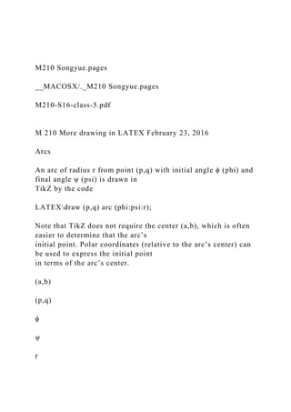
  • 1. M210 Songyue.pages __MACOSX/._M210 Songyue.pages M210-S16-class-5.pdf M 210 More drawing in LATEX February 23, 2016 Arcs An arc of radius r from point (p,q) with initial angle ϕ (phi) and final angle ψ (psi) is drawn in TikZ by the code LATEXdraw (p,q) arc (phi:psi:r); Note that TikZ does not require the center (a,b), which is often easier to determine that the arc’s initial point. Polar coordinates (relative to the arc’s center) can be used to express the initial point in terms of the arc’s center. (a,b) (p,q) ϕ ψ r
  • 2. p = a + r cosϕ q = b + r sinϕ In tikzpicture environment enter draw ({a+r*cos(phi)},{b+r*sin(phi)}) arc (phi:psi:r); for the specific values of a, b, r, ϕ (phi) and ψ (psi). LATEX According to the TikZ’s manual, by default arcs are drawn in positive (counter-clockwise) direction, assuming initial angle ϕ to be smaller than ψ. However, I have been able to draw arcs in negative (clockwise) direction by choosing an initial angle larger than final angle. Precise Label Positioning The relative positions above, below, left, right, above left, above right, below left, and below right, provide positioning relative to the node (indicated by the dot) as illustrated in the following figures. below above left right above left below left
  • 3. above right below right While it is possible to adjust the separation between label and node, it is not that easy to adjust the angle (the above provide label placement only for angles in multiples of 45◦). The following will work to place the label (that is its center) at the the indicated position: precise distance s at relative angle θ from the position of the node. node lab el s node coordinates (nx,ny) label coordinates (lx, ly) θ To place label at the above mentioned position use the code (where θ is theta degrees): M 210 — February 23, 2016 page 44 LATEXdraw ({nx + s*cos(theta)}, {ny + s*sin(theta)}) node {label}; To rotate the label as in the above illustration, use code:
  • 4. LATEXdraw ({nx + s*cos(theta)}, {ny + s*sin(theta)}) node {rotatebox{theta}{label}}; Special Triangles In trigonometry the triangles with degrees 45-45-90 and 30-60- 90 provide exact values for the trigono- metric functions. It is quite easy to obtain the exact values of angles of 15 and 75 degrees from those of 30 degrees by half- and double-angle formulas and other trigonometric identities, however, these values can also be obtained from the following figure containing an equilateral triangle in a square with sides equal to 2. 1 The Regular Pentagon. Use trigonometric functions to draw a regular pentagon with its lower side along the line segment from (−1,0) to (1,0). Start by drawing this line segment. LATEXbegin{center} begin{tikzpicture}[scale=2] draw[line width=1.2pt] (-1,0) -- (1,0); end{tikzpicture} end{center} Extend the line segment on both sides by adding the following code. LATEXdraw[line width=1.2pt] (1,0) -- ({1+2*cos(72)},{2*sin(72)});
  • 5. draw[line width=1.2pt] (-1,0) -- ({-1-2*cos(72)},{2*sin(72)}); Close the top of the pentagon, using angles denoted in the desired figure on the following page, by adding the following code. LATEXdraw[line width=1.2pt] ({1+2*cos(72)},{2*sin(72)})--(0,{2*sin(72)+2*sin(36)})--({-1- 2*cos(72)},{2*sin(72)}); Of course we can shorten the code by placing it all in one string using --cycle to close the pentagon’s path. M 210 — February 23, 2016 page 45 Now add the following lines to provide a coordinate system. LATEXdraw[gray] (-2,0)--(2,0); draw[gray] (0,-.25)--(0,3.35); Add the second gray horizontal line. Color and label the indicated angles. The yellow angle with the x-axis was obtained by the following code. LATEXdraw[fill=yellow!50] (1,0)--(1.55,0) arc (0:72:0.55) -- cycle; Use this as an example to draw the other angles. 108◦ 72◦
  • 6. 72◦ 36◦ 1 1/2 cos(72◦) cos(36◦) From the figure we see cos(36◦) = 1 2 + cos(72◦). Using the double angle formula for the cosine we have cos(36◦) = 1 2 + 2 cos2(36◦) − 1, which can be rewritten as 4 cos2(36◦) − 2 cos(36◦) − 1 = 0. Because cos(36◦) > 0, with the help of the quadratic formula we conclude cos(36◦) = 2 +
  • 7. √ 4 − 4(4)(−1) 8 = 2 + √ 20 8 = √ 5 + 1 4 . It follows that cos(72◦) = √ 5 − 1 4 . See TikZercise 3 for an alternative derivation. Construction Regular Pentagon. Draw a unit circle, and let A and B be the points (0,1) and (−1,0), respectively.
  • 8. M 210 — February 23, 2016 page 46 B O A Let C be the midpoint of OB. Then by the Pythagorean Theorem we have AC2 = (1/2)2 + 12 = 5/4 =⇒ AC = 1 2 √ 5. B O A C Use AC as length for a pentagon, constructed as indicated in the following figure. M 210 — February 23, 2016 page 47 B
  • 9. O A C D EF Homework 4 TikZercises. Draw the following in a LATEX document using TikZ: 1. Draw the following proof of the Pythagorean Theorem. a b c c c c b a b a a b
  • 10. a a a b b b M 210 — February 23, 2016 page 48 2. Draw the figure from page 44 with all angles labelled, and use the figure to find the exact values of cos, sin and tan at angles 15◦ and 75◦. 3. Draw a right-angled triangle with angles 72◦ and 18◦ whose side adjacent angle 72◦ has length 1 as shown in the adjacent figure. To determine the exact value of hypotenuse x, first put two such triangles together as indicated in the following figure. Next, extend the above tri- angles’ base, mark a point E length x to the left of A along the base and complete a larger triangle BDE as shown in the following figure. 72◦
  • 11. 18◦ x 1A B C 72◦ 72◦ 18◦ 18◦ x 1 1x A B C DE Answer the following questions in your LATEX document: (a) Find the missing angles ∠ AEB and ∠ ABE. (b) Show that triangles DBE and ADB are similar. (c) Using the similarity of triangles DBE and ADB, set up an equation for x and solve this equation. (d) Find the missing sides and angles in the following two special right triangles, then draw them showing all sides and angles.
  • 12. M 210 — February 23, 2016 page 49 72◦ 18◦ 1A C B E C B 4. Draw the following figure with missing angles (indicated by arcs) and line segments filled in, and use this information to find identities for cos(α + β) and sin(α + β). [Use optional argument rotate=ang in draw for appropriate angle ang (in degrees) to rotate the line segments to denote a right angle.] α β 1 M 210 — February 23, 2016 page 50
  • 13. 5. On the legs of angle ∠ ABC points P , Q, R and S are so that all five blue segments are equal (BP = PS = SR = RQ = BQ). Draw this figure and show that ∠ ABC = 36◦. C AB R S P Q 6. The following figure 1/2 1/4 1/8 1/16 1/32 1/64 1/128 1 256 shows that
  • 15. 256 + · · · = 1. Using summation notation, the above states that ∞ ∑ k=1 1 2k = 1. M 210 — February 23, 2016 page 51 7. Draw the following figure and typeset the derivation of the Law of Cosines following the figure. θ a c b acosθ b − acosθ a si n θ The Pythagorean Theorem applied to the right-angled triangle
  • 16. results in c2 = (asinθ)2 + (b − acosθ)2 = a2 sin2 θ + b2 + a2 cos2 θ − 2ab cosθ = a2(cos2 θ + sin2 θ) + b2 − 2ab cosθ = a2 + b2 − 2ab cosθ. 8. Draw the following figure. θ θ 1 cos θ sin θ cos2 θ sin2 θ θ co s θ sin θ co s θ
  • 17. sin θ Behold: cos 2θ = cos2 θ − sin2 θ, sin 2θ = 2 cosθ sinθ. 9. Draw the following figure, and typeset the conclusions. M 210 — February 23, 2016 page 52 A BC P θ θ 1 2θ Q cos 2θ sin 2θ cos θ
  • 18. cos θ Considering right △APQ, it follows from the figure that sinθ = sin 2θ 2 cosθ , cosθ = 1 + cos 2θ 2 cosθ , from which the identities sin 2θ = 2 cosθ sinθ, cos 2θ = 2 cos2 θ − 1. follow easily. Submit Homework 4 by 3:00pm on Tuesday, March 1, to Moodle. Please put course, your last name, and homework number in the name of the file you submit (using a file name like M210-HW4-name). __MACOSX/._M210-S16-class-5.pdf M210-S16-class-7.pdf
  • 19. M 210 Introduction to Mathematica March 8, 2016 Creator of Mathematica British-born Stephen Wolfram received a Ph.D. in particle physics from the California Institute of Technology at age 20. In 1986 Wolfram founded the Center for Complex Systems Research at the University of Illinois at Urbana-Champaign and started to develop the computer algebra system Mathematica, which was first released in 1988, when he left academia. In 1987 he co-founded a company called Wolfram Research which continues to develop and market the program. Stephen Wolfram Formatting Stylesheet from Format from the menu contains several stylesheets that can be used to change the appearance of a Mathematica Notebook. Title and sections header can be selected from Style from the menu. Clicking the plus (+) symbols following an output cell will bring up a window from which one can select Plain text or Other style text to include in the Notebook. Notational Conventions During a Mathematica session input cells and output cells are labelled In[1], Out[1], In[2], Out[2], In[3], Out[3], etc. Input cells are evaluated by either the enter key or the shift-return key.
  • 20. Built-in Mathematica commands and functions always begin with a capital letter. It is good practice to use lowercase letters for user defined objects. Function arguments are always enclosed by square brackets [ ]. Parentheses ( ) are used to group objects together, and to establish priority of opera- tions. Standard arithmetic operations are +, -, *, /, and ^. A space is interpreted as multiplication: xy is not the same as x*y, but the latter is the same as x y. Variable names cannot start with numbers, but otherwise numbers can occur, for example as subscripts. Greek letters can be entered and used, and something like ∆x can be a single variable. Comments are delimited by (* and *). The symbol % refers to the previous output, %% to the second- previous output, etc. It is also possible to refer to the output following Out[n] by using Out[n] or simply by %n. Output can be given in TraditionalForm, which is an attempt to match traditional mathematical notation. While it is possible to use TraditionalForm also for input, it is better to use StandardForm, which is the default for both input and output. Calculator When he was ten years old, the calculating prodigy Truman Henry Safford (1836–1901) of Royalton, Vermont, was once asked to square, in his head, the number 365,365,365,365,365,365. His church leader reports, “He flew around the room like a top, pulled his pantaloons over the tops of his boots, bit his hands, rolled his eyes in their sockets, sometimes smiling and talking, and then seeming to be in
  • 21. agony, until in not more than a minute said he, 133,491,850,208,566,925,016,658,299,941,583,225”[1]. • Verify Safford’s answer using Mathematica. Mathematical Constants Mathematica contains several mathematical constants such as Pi for π, E for Euler’s number e, I for the imaginary number i = √ −1, and GoldenRatio for the golden ratio. M 210 — March 8, 2016 page 63 Some of these constants can be displayed similarly to the usual notation, such as π, e, and i, by making use of the escape key Esc , as follows: Traditional form Key sequence π Esc p Esc e Esc ee Esc i Esc ii Esc Likewise, superscripts and subscripts can be obtained combining the control key with ^ and -. Traditional form Key sequence x2 x Ctrl 6 2 >
  • 22. x1 x Ctrl - 1 > • Use Mathematica to evaluate eπi (make sure to leave space between the two symbols in the exponent; the answer should be −1). The letters N and D cannot be used as names for user defined objects; they are built-in commands: the first for numerical approximation, the second for differentiation. Mathematica displays only six decimals by default when the numerical approximation N is applied. To get m digits of expr enter N[expr,m]. • Have Mathematica calculate 100 digits of π and of e. • Which is larger πe or eπ? (The first computes to less than 23, the second to a number larger than 23.) The StandardForm of Infinity can also be obtained using the escape key. Greek letters can be input using the escape key. The following table contains keyboards shortcuts for some common symbols. Key sequence Result Full Name Esc a Esc α [Alpha] Esc D Esc ∆ [CapitalDelta] Esc inf Esc ∞ [Infinity] Esc e Esc ǫ [Epsilon] Esc ce Esc ε [CurlyEpsilon]
  • 23. Esc deg Esc ◦ [Degree] Esc -> Esc → [Rule] Esc => Esc ⇒ [Implies] The golden ratio is often denoted by the Greek letter phi in honor of the Greek sculptor Phidias (ca 480 BC–430 BC). • Use the letter ϕ for the golden ratio (can be input in Mathematica as Esc cphi Esc ), then simplify ϕ2 − ϕ. In[1]:= ϕ = GoldenRatio In[2]:= Simplify[ϕ2 − ϕ] In[3]:= Solve[x^2 - x == 1] • What can you conclude about ϕ? The golden ratio is the largest root of the above equation, which is the number ϕ = √ 5 + 1 2 . This is the constant GoldenRatio in Mathematica (the other root of the above equation is the reciprocal of this constant).
  • 24. M 210 — March 8, 2016 page 64 Symbolic Calculator If a variable var has been assigned a value this can be undone by using Clear[var] or, equivalently, inputting var =.. Once a variable has been assigned a value, Mathematica will substitute that value in all calculations of the session. For example, suppose we have calculated an expression to be 5 − 3x + x3, and now wish to evaluate this at x = 2. Far easier than to assign value 2 to variable x, then evaluate the expression, and finally clearing x, as indicated in the following sequence of code Out[1]= 5 - 3 x + x^3 In[2]:= x=2 Out[2]= 2 In[3]:= %% Out[3]= 7 In[4]:= x=. would be to substitute the value of x into the given expression using /. followed by a value assignment to x using a right arrow as follows. Out[1]= 5 - 3 x + x^3 In[2]:= % /. x → 2 Out[2]= 7 Substitution using /. makes it unnecessary to unclear the variable. Lists
  • 25. Mathematica uses braces { and } for ordered lists, with the elements contained in the lists separated by commas. If L denotes a list, then L[[k ]] gives its kth entry. The double square brackets are entered using the escape key: Esc [[ Esc gives [[ and ]] is obtained similarly. Note that the escaped double square brackets only serve an esthetic purpose (visually showing the components as functions of the list); using plain double brackets [[ and ]] will work as well (and saves key strokes). In[1]:= L = {1, 8, 28, 56, 70, 56, 28, 8, 1} Out[1]= {1, 8, 28, 56, 70, 56, 28, 8, 1} In[2]:= L[[4]] Out[2]= 56 The command Table can be used to create lists generated by formulas. For example In[3]:= T = Table[i^2, {i, 10}] Out[3]= {1, 4, 9, 16, 25, 36, 49, 64, 81, 100} These lists can be manipulated with the various arithmetic operators. • Investigate the result of adding and multiplying these lists, and squaring each of them. Lists can be plotted using the ListPlot command: In[4]:= ListPlot[L] The built-in function Prime gives the prime numbers in order.
  • 26. We can generate a list of the first 1000 prime numbers: In[5]:= Table[Prime[i], {i, 1000}] M 210 — March 8, 2016 page 65 Sums and Series Evaluate some partial sums of the series ∑∞ n=1 1/n 2. In[1]:= Sum[1/n2, {n, 1, 10}] In[2]:= Sum[1/n2, {n, 1, ∞}] Integral Integrals are evaluated similarly to sums. Evaluate the integral ∫ 1 0 x4(1 − x)4 1 + x2 dx by entering the following. In[1]:= Integrate[x^4(1 - x)^4/(1 + x^2), {x, 0, 1}]
  • 27. The answer is 22 7 − π. The above integral provides a means of estimating the error in the approxi- mation π ≈ 22 7 ; see the next example. Plotting We can plot the function in the above integral as follows. In[1]:= Plot[x^4(1 - x)^4/(1 + x^2), {x, 0, 1}] Locate the maximum of the above function, by setting its derivative equal to zero to find its critical point. Use this to estimate the integral, and thus obtain a bound for the exact answer of the integral obtained earlier. Following are the first steps of the above procedure. In[2]:= D[x^4(1 - x)^4/(1 + x^2), x] In[3]:= Solve[% == 0,x] In[4]:= x^4 (1 - x)^4/(1 + x^2) /. %[[7]] In[5]:= N[%] The computed result of 0.00315543 gives an upperbound for the integral ∫ 1 0 x4(1−x)4 1+x2 dx, and thus
  • 28. an upperbound for the error in the approximation π ≈ 22 7 . Functions Functions are defined using delayed assignment := and indicating variable by following them with underscores. In[1]:= f[x_]:=x^2 In[2]:= f[a+b+c] // Expand Note that if Fcn is a function, expr // Fcn is short-hand for Fcn[expr]. In[3]:= (f[x+h]-f[x])/h // Simplify M 210 — March 8, 2016 page 66 Animation Define the cycloid by In[1]:= Cycloid[t_] := {t - Sin[t], 1 - Cos[t]} This is a parametric curve that can be plotted using ParametricPlot: In[2]:= ParametricPlot[Cycloid[t], {t, 0, 2 Pi}] The following creates a simple animation. Animate[Graphics[{ {EdgeForm[{Black, Thick}], Yellow, Disk[{t, 1}]},
  • 29. Line[{{-1, 0}, {7, 0}}], {Thick, Line[{{t, 1}, Cycloid[t]}]}, Disk[Cycloid[t], .075]}], {t, 0, 2 Pi}] Immediate versus Delayed Assignment An immediate assignment is made using =, while := is used for a delayed assignment. If we set variable x equal to 2 by using as input x=2, then variable x will be replaced by the number 2. The function Random with empty argument generates a random number between 0 and 1. In[1]:= x = Random[] In[2]:= {x, x, x} Compare the output generated by the above code with that of In[3]:= y := Random[] In[4]:= {y, y, y} An Example of Simplification Use Mathematica to simplify ( √ 6 − √ 2)( √
  • 30. 3 + √ 2) − 2 √ ( √ 6 − √ 2)( √ 3 + √ 2) . The command Simplify has little effect. We can use the command FullSimplify, which simplifies the given expression. Mathematica simplifies the expression to an expression containing nested radicals, which it does not simply any further. Help Mathematica to see if the expression can be further simplified to a number that involves 4 √ 2 and its reciprocal. [Suggestion: consider the square of 21/4 − 2−1/4.]
  • 31. In[1]:= q=((Sqrt[6]-Sqrt[2])(Sqrt[3]+Sqrt[2])-2)/Sqrt[(Sqrt[6]- Sqrt[2])(Sqrt[3]+Sqrt[2])] In[2]:= Simplify[q] In[3]:= FullSimplify[q] M 210 — March 8, 2016 page 67 Using FullSimplify Mathematica arrives at the answer √ 6 √ 2 − 8 (Mathematica displays this in different order, use TraditionalForm[%] to see identical output by Mathematica). Can this answer possibly be simplified? Let’s use Mathematica to calculate the square of 4 √ 2−1/ 4 √ 2. Using fractional exponents we enter this in Mathematica as follows. In[4]:= (2^(1/4)-2^(-1/4))^2 // Expand The answer is reminiscent of the earlier output above. In fact, let’s have Mathematica compare the result of the last computation with the expression under the square root of its answer to the
  • 32. FullSimplify command: In[5]:= %/(-8 + 6 Sqrt[2]) // Expand Mathematica’s answer shows that twice the number 4 √ 2 − 1/ 4 √ 2 is √ 6 √ 2 − 8, so that our origi- nal expression (in Mathematica stored in variable q) would be equal to 2( 4 √ 2 − 1/ 4 √ 2). Let’s use Mathematica to verify this: In[6]:= FullSimplify[q - 2(2^(1/4)-2^(-1/4))] The calculation confirms that we have found a simplified answer for the original fraction: ( √
  • 33. 6 − √ 2)( √ 3 + √ 2) − 2 √ ( √ 6 − √ 2)( √ 3 + √ 2) = 2 ( 4 √ 2 − 1 4 √
  • 34. 2 ) . Using the rules of exponents we can rewrite the right-hand side of the above formula as 2 · 21/4 − 2 · 2−1/4 = 25/4 − 23/4. Mathematica’s command FullSimplify can also be used to confirm this result: In[7]:= FullSimplify[q - (2^(5/4)-2^(3/4))] We have the following pretty simplification: ( √ 6 − √ 2)( √ 3 + √ 2) − 2 √ ( √ 6 −
  • 35. √ 2)( √ 3 + √ 2) = 25/4 − 23/4. This example shows that while a computer algebra system (CAS) is very useful in simplifying complicated expressions, it may be necessary to provide intelligent coaching to get at expressions the CAS may not directly supply. Special Trigonometric Values Use Mathematica to verify the following formula for the cosine (arrived at by several applications of double-angle formulas): cos 4θ = 1 − 8 sin2 θ + 8 sin4 θ. (1) Simplify[Cos[4 [Theta]] - 1 + 8 Sin[[Theta]]^2 - 8 Sin[[Theta]]^4] Observing that 90◦ − 18◦ = 72◦ = 4(18◦), we easily see that sin(18◦) = cos 4(18◦), so by (1) x = sin(18◦) satisfies the equation x = 1 − 8x2 + 8x4. (2) Use Mathematica to solve (2), and deduce from Mathematica’s answer the exact value of sin(18◦). Verify your answer using Mathematica.
  • 36. There are several ways to solve the above polynomial equation. First it is easy to see that x = 1 is a solution so that x − 1 is a factor of the polynomial 8x4 − 8x2 − x + 1, and we can divide to obtain the quotient: M 210 — March 8, 2016 page 68 (8x^4-8x^2-x+1)/(x-1) // Simplify The quotient is 8x3 + 8x2 − 1. We can has Mathematica evaluate this at −1/2 by entering: 8x^3+8x^2-1 /. x->-1/2 Since the result is 0 also x − (−1/2) = x + 1/2 is a factor, so also 2x + 1. Divide this out: (8x^3+8x^2-1)/(2x+1) // Simplify The resulting quotient is 4x2 +2x−1, and x = sin(18◦) is a solution of the equation 4x2 +2x−1 = 0. Using the quadratic formula we get x = −1± √ 5 4 . Because sin(18◦) > 0 we conclude that sin(18◦) = √ 5 − 1 4
  • 37. . An alternative is to factor the given polynomial 8x4 − 8x2 − x + 1: Factor[8x^3+8x^2-1] Another alternative is to use Mathematica’s built-in solver: Solve[8x^3+8x^2-1,x] Using the subtraction formula for the sine and the exact values for sin(15◦) and cos(15◦) it is now easy to find an exact values for sin(3◦) and cos(3◦); see the first homework problem on page 136. Another Example of Simplification Use Mathematica to show that √ 5(1 + 5 √ 4) = 5 √ 2 + 5 √ 8 + 5 √
  • 38. 16 − 1. We enter the expressions into variables a and b in Mathematica: a=Sqrt[5(1+Surd[4,5])] b=Surd[2,5]+Surd[8,5]+Surd[16,5]-1 We can have Mathematica numerically approximate each of these quantities: N[a] N[b] The above calculation does not establish the above formula (the calculation merely shows that the quantities are close to each other). To show the formula we need to use algebra. The following computes the square of quantity b: b^2 Expand[%] Since b is positive, validity of the formula is now established. A Third Example of Simplification Use Mathematica to simplify 3 √ 2 + √
  • 39. 5 + 3 √ 2 − √ 5. The numbers a = 3 √ 2 + √ 5 and b = 3 √ 2 − √ 5 satisfy a3 = 2 + √ 5 and b3 = 2 − √ 5, so a3 + b3 = 4. Before we enter these into Mathematica, lets do some algebra:
  • 40. M 210 — March 8, 2016 page 69 Clear[a,b] (a+b)^3 // Expand /. a^3+b^3->4 Factor waht remains after subtracting 4: Factor[%-4] Now observe that ab is easily computed, because (2 + √ 5)(2 − √ 5) = −1. So x = a + b satisfies the equation x3 = 4 − 3x, that is x3 + 3x − 4 = 0. The calculation Solve[x^3+3x-4==0] shows that this cubic equation has one real real root, thus 3 √ 2 + √ 5 + 3 √
  • 41. 2 − √ 5 = 1, a result that can also be obtained using Mathematica’s FullSimplify instead of Simplify (which does not do anything with this input). Some Plotting Options The AspectRatio is by default set to the reciprocal of the golden ratio. Turning it to Automatic will set the same aspect ratio along the x- and y-axis. Test with the function y = √ 1 − x2, −1 ≤ x ≤ 1. Compare Plot[Sqrt[1-x^2], {x, -1, 1}] and Plot[Sqrt[1-x^2], {x, -1, 1}, AspectRatio -> Automatic] A list of functions can be plotted together, for example Plot[{Sin[x], Sin[2x]}, {x, 0, 2 Pi}] It is possible to have the plot display labels when the cursor is placed over one of the functions graphed. This is done using the function Tooltip, which takes two arguments: first the function, and second the label, entered between quotation marks. Example:
  • 42. Plot[{Tooltip[Sin[x], "sin x"], Tooltip[Sin[2 x], "sin 2x"]}, {x, 0, 2 Pi}] The above plot has the same appearance as the one before, but see what happens when the cursor is moved over one of the graphs. We can change the color and thickness of the graph by using the option PlotStyle, for example PlotStyle->{Thickness[0.005], Red}. If there is a list of functions, PlotStyle needs to be assigned to a list. Plot[{Sin[x], Sin[2x]}, {x, 0, 2 Pi}, PlotStyle -> {{Thickness[0.005], Red}, {Thickness[0.0075], Blue}}] We can add axes labels and ticks along the x-axis at π/2, π, 3π/2, 2π by adding AxesLabel and Ticks options: Plot[{Sin[x], Sin[2x]}, {x, 0, 2 Pi}, PlotStyle -> {{Thickness[0.005], Red}, {Thickness[0.0075], Blue}} AxesLabel -> {x, y}, Ticks -> {{Pi/2, Pi, 3 Pi/2, 2 Pi}, Automatic}] M 210 — March 8, 2016 page 70 Note that Ticks is assigned a list of specification for the first
  • 43. and second axis. In the above example Automatic is chosen for the ticks along the second axis. Another possibility is None, which produces no ticks. Note that a list of values such as π/2, π, 3π/2, 2π is more easily specified using Range[a,b,c], where a and b are the first and last number and c denotes the increment. Enter the following in Mathematica: Range[Pi/2, 2Pi, Pi/2] We can set Frame to True to create a frame around the plot, and we can use FrameTicks to specify ticks along the edges of this frame. Note that FrameTicks takes a list of tick specifications for the pairs of vertical left and right edges, followed by the horizontal bottom and top edges. Plot[{Sin[x], Sin[2 x]}, {x, 0, 2 Pi}, PlotStyle -> {{Thickness[0.005], Red}, {Thickness[0.0075], Blue}}, Frame -> True, Axes -> True, FrameTicks -> {{Range[-1, 1, 1/2], None}, {Range[0, 2 Pi, Pi/6], None}}] Gridlines can be added using GridLines. One option for GridLines is Automatic, but one can also specify the exact location of the gridlines, as in the following example, which also specifies the style of the gridlines as an ordered pair (replace one of the colors Green by some other other color to see the order).
  • 44. Plot[{Sin[x], Sin[2 x]}, {x, 0, 2 Pi}, PlotStyle -> {{Thickness[0.005], Red}, {Thickness[0.0075], Blue}}, Frame -> True, Axes -> True, FrameTicks -> {{Range[-1, 1, 1/2], None}, {Range[0, 2 Pi], Pi/6, None}}, GridLines -> {Range[0, 2 Pi, Pi/6], Range[-1, 1, 1/2]}, GridLinesStyle -> {{Thin, Green}, {Thin, Green}}] There are a lot more options for Plot. Enter the following in Mathematica to see all option: Options[Plot] Help for a command is provided executing the command following ?, for example ? Plot Piecewise Defined Functions Piecewise defined functions can be obtained using Piecewise[{{expr1,cond1},{expr2,cond2},...,{exprn,condn}}], where exprj are expressions and condj are conditions, for j = 1, 2, . . . , n. Examples: Plot[Piecewise[{{-x, x < 0}, {x, x >= 0}}], {x, -5, 5}] Plot[Piecewise[{{Sqrt[-x], x < 0}, {Sqrt[x], x >= 0}}], {x, -5,
  • 45. 5}] Let’s define a pulse function, and plot it: ClearAll[f] f[x_] := Piecewise[{{1 + x, -1 <= x < 0}, {1 - x, 0 <= x <= 1}}] Plot[f[x], {x, -5, 5}] The displayed plot is lousy at best. We need to help Mathematica with the range of this function, which is done using PlotRange. Plot[f[x], {x, -5, 5}, PlotRange -> {0, 1}] M 210 — March 8, 2016 page 71 The plot produced by the above is better, but the aspect ratio could be improved. Plot[f[x], {x, -5, 5}, PlotRange -> {0, 1}, AspectRatio -> Automatic] This is better, but the automatic ticks along the vertical axis are cluttered, so we remove them or specify them as follows. Plot[f[x], {x, -5, 5}, PlotRange -> {0, 1}, AspectRatio -> Automatic, Ticks -> {Automatic, {0, 1}}] Now that we have a single pulse function, we can see what
  • 46. happens when we translate. In the same coordinate system as f draw the graphs of y = f(x + 3) and y = f(x − 3), and identify these functions in the plot using Tooltip starting from: Plot[{f[x], f[x + 3], f[x - 3]}, {x, -5, 5}, PlotRange -> {0, 1}, AspectRatio -> Automatic, Ticks -> {Automatic, None}] Since the pulses do not overlap, the following function has the same graph: Plot[f[x] + f[x + 3] + f[x - 3], {x, -5, 5}, PlotRange -> {0, 1}, AspectRatio -> Automatic, Ticks -> {Automatic, None}] Sound Mathematica can also produce sound, which it treats analogous to graphics. The following plays a pure tone with frequency 440 Hertz for one second. In[1]:= Play[Sin[2 Pi 440 t], {t, 0, 1}] • Play some pure tones with other frequencies. Using the idea of the previous section we can create a function that when played by Mathematica (using Play) produces a complete octave of pure notes. Using Data Sets Mathematica can call up massive data sets maintained by Wolfram Research, and these data sets can be used to define functions.
  • 47. The following yields a list of CountryData. In[4]:= CountryData["Properties"] We can use this to display the flag and present population of countries, for example China. In[5]:= Graphics[CountryData["China", "Flag"]] In[6]:= CountryData["China", "Population"] In[7]:= CountryData["China", "Area"] M 210 — March 8, 2016 page 72 The following function defines the population density of a country, indicated by the variable c, and is used to calculate the population density of China. In[8]:= popdensity[c ] := CountryData[c, "Population"]/CountryData[c, "Area"] In[9]:= popdensity["China"] The resulting answer is the population density in number of people per square kilometer. References [1] Clifford A. Pickover, A Passion for Mathematics: Numbers, Puzzles, Madness, Religion, and the Quest for Reality, John Wiley & Sons, 2005. M 210 — March 8, 2016 page 73
  • 48. Homework 6 This assignment consists of only Mathematica problems. Solution s of the problems should be given in a single Mathematica notebook displaying the requested formulas and graphics (please put your name, the assignment number and date on the top of your Mathematica notebook). 1. (a) Use Mathematica to find the exact values of sin 18◦, cos 18◦, sin 15◦, and cos 15◦. (b) Use the formula sin(u − v) = sin u cos v − cos u sin v to find an exact value for sin 3◦. (c) Find an exact value for cos 3◦. 2. The Indian mathematician Ramanujan discovered many formulas for denesting radicals. Use Mathematica to verify the following formulas found by Ramanujan:
  • 49. (a) 3 √ 3 √ 2 − 1 = 3 √ 1/9 − 3 √ 2/9 + 3 √ 4/9. (b) 6 √
  • 50. 7 3 √ 20 − 19 = 3 √ 5 3 − 3 √ 2 3 . Srinivasa Ramanujan (1887–1920)(c) √
  • 51. 3 √ 28 − 3 √ 27 = 1 3 ( 3 √ 98 − 3 √ 28 − 1 ) . (d)
  • 52. √ 3 √ 5 − 3 √ 4 = 1 3 ( 3 √ 20 + 3 √ 2 − 3 √
  • 53. 25 ) . 3. Plot a graph of the function y = tan(sin x) − sin(tan x) over the interval [−π, π]. 4. (a) Plot the graph of the function f(x) = x(1 − x) 1 + x2 , 0 ≤ x ≤ 1. (b) Find exact expressions for the maximum value of f and where this value is obtained. (c) Use derivative(s) to determine the graph’s concavity. 5. Use Mathematica to compute and rank the population densities of the following countries Argentina, Canada, China, Germany, Netherlands, US.
  • 54. 6. [Extra Credit] Construct a function that when played by Mathematica (using Play) produces a complete octave of pure notes. Submit Homework 6 by 3:00pm on Tuesday, March 15, to Moodle. Please put course, your last name, and homework number in the name of the file you submit (using a file name like M210-HW6-name.nb). __MACOSX/._M210-S16-class-7.pdf M210-S16-class-8.pdf M 210 Plotting and Graphics in Mathematica March 15, 2016 We continue our discussion of Mathematica and cover more plotting and graphics. The last part of the handout contains more material on LATEX: cropping of pictures included with the graphicx package, and some further formatting.
  • 55. Contents 1 More Plotting in Mathematica 74 1.1 Plot Options . . . . . . . . . . . . . . . . . . . . . . . . . . . . . . . . . . . . . . . . . . . . . 74 1.2 Changing Directory . . . . . . . . . . . . . . . . . . . . . . . . . . . . . . . . . . . . . . . . . . 74 1.3 Points and Lines . . . . . . . . . . . . . . . . . . . . . . . . . . . . . . . . . . . . . . . . . . . 75 1.4 Tangent Lines . . . . . . . . . . . . . . . . . . . . . . . . . . . . . . . . . . . . . . . . . . . . . 75 1.5 Polar Curves . . . . . . . . . . . . . . . . . . . . . . . . . . . . . . . . . . . . . . . . . . . . . 77 1.6 Implicit Curves . . . . . . . . . . . . . . . . . . . . . . . . . . . . . . . . . . . . . . . . . . . . 77 1.7 Regions . . . . . . . . . . . . . . . . . . . . . . . . . . . . . . . . . . . . . . . . . . . . . . . . 80
  • 56. 2 Cropping Images, Image Conversion and Graphics Paths 80 2.1 Cropping Images . . . . . . . . . . . . . . . . . . . . . . . . . . . . . . . . . . . . . . . . . . . 80 2.2 Graphics Path . . . . . . . . . . . . . . . . . . . . . . . . . . . . . . . . . . . . . . . . . . . . 82 3 Further Formatting of LATEX Documents 83 1 More Plotting in Mathematica 1.1 Plot Options The following table lists several useful options for Plot. Some options for Plot option name default value description AspectRatio 1/GoldenRatio ratio of width to height; set to Automatic to have equal units in horizontal and vertical direction Axes True axes are drawn
  • 57. AxesLabel None place labels along axes. Use {"x","y"} to get these labels Exclusions Automatic points to exclude LabelStyle {} style specification for labels (default empty). Filling None filling to insert under each curve FillingStyle Automatic style to use for filling PlotRange {Full,Automatic} range of variables to include. ColorFunction Automatic determines color of the surface PlotLabel None label for plot PlotLegends None legends for curves PlotStyle Automatic graphics directives for style of each surface ToolTip specifies an explicit tooltip label for a curve Pages 75–80 discuss several examples. We will discuss further examples after first showing how to graph points and lines (so that these can be included in further examples). 1.2 Changing Directory Mathematica saves and exports graphics files to it current directory. The command SetDirectory can be used to change this directory to a more convenient
  • 58. folder. To change it to the subfolder mma of folder M210 on a flash drive labeled F, input the following into Mathematica: M 210 — March 15, 2016 page 75 SetDirectory["F:M210mma"] For Mac users, setting Mathematica’s current directory the subfolder mma of folder M210 on a flash drive named USB20FD, input the following into Mathematica: SetDirectory["/Volumes/USB20FD/M210/mma/"] Pictures saved or exported from Mathematica will then be stored in the subfolder mma of folder M210 on the flash drive. 1.3 Points and Lines Points and Lines are plotted using the functions Point and Line with appropriate arguments in the Graphics command.
  • 59. The code Graphics[Point[{1, 0}]] draws a point at (1, 0). There is no visible difference in output if the coordinates are changed, because Mathematica automatically centers the graphic at the only graphical element. More than one point can be plotted by listing the coordinates of the points. See what happens executing Graphics[Point[{{0, 0}, {1, 0}, {1/2, 1/2}}]]. The size of the point can be set by PointSize, which takes as possible arguments Large, Medium, Small, or numbers. Color can be specified by listing it as well, using capital letter, such as in Blue, Red, Yellow, LightGreen, etc. These size and color attributes can be applied to the list of points, as is the case in Graphics[{PointSize[Large], Red, Point[{{0, 0}, {1, 0}, {1/2, 1/2}}]}] If we want different size and colors for the points, we can specify this as in the following example: Graphics[{{PointSize[Large], Red, Point[{0, 0}]},
  • 60. {PointSize[Medium], Blue, Point[{1, 0}]}, {PointSize[0.02], Green, Point[{1/2, 1/2}]}}] Line (segments) are specified by points between which they are to be drawn. These points are to be given in a list of ordered pairs, such as in the following example. Graphics[Line[{{0, 0}, {2, 0}}]] More segments can be included by including more points in the list, for example Graphics[Line[{{0, 2}, {0, 0}, {2, 0}}]] To draw coordinate axes we can use Arrow instead of Line, but we need of course have a pair of points as argument (since an arrow goes from a begin point to an end point): Graphics[{Arrow[{{0, 0}, {2, 0}}], Arrow[{{0, 0}, {0, 2}}]}] Line (or arrow) thickness and color can be specified similarly to how these attributes were added to
  • 61. points, for example: Graphics[{Thick, Blue, Line[{{0, 2}, {0, 0}, {2, 0}}]}] We will later discuss other primitive graphical objects, the above suffices to create plots that involve tangent lines. 1.4 Tangent Lines Start by plotting the function y = sin x over the interval [0, 2π]. Define a to be equal to π/3. The point (a, sin a) can then be plotted together with the graph of the function, by placing the Plot for the graph and Graphics[Point[{a, Sin[a]}] together using the Show function as follows: M 210 — March 15, 2016 page 76 a = Pi/3; Show[Plot[Sin[x], {x, 0, 2 Pi}, Ticks -> {Range[0, 2 Pi, Pi/2], Automatic}],
  • 62. Graphics[{PointSize[0.01], Red, Point[{a, Sin[a]}]}]] Note that the graphical elements are drawn in the order in which they are listed as argument of Show, and since we want to see the point on the graph, it is listed after the graph of the function. Before we add the tangent line to the graph, let’s animate the above over a: Manipulate[ Show[Plot[Sin[x], {x, 0, 2 Pi}, Ticks -> {Range[0, 2 Pi, Pi/2], Automatic}], Graphics[{PointSize[0.015], Red, Point[{a, Sin[a]}]}]], {a, 0, 2 Pi}] We can now add the tangent line by entering the function y = sin a+cos a(x−a) as a second function. Since we want to animate the resulting plot we put in a range specification (since the added line will cause Mathematica to change range for different values of a), and we color the tangent line (second
  • 63. plot) in the same color as the point parametrized by a. The following code should accomplish this: a = Pi/3; Show[ Plot[{Sin[x], Sin[a] + Cos[a] (x - a)}, {x, 0, 2 Pi}, PlotRange -> {-2, 2}, Ticks -> {Range[0, 2 Pi, Pi/2], Automatic}, PlotStyle -> {{Thick, Blue}, {Thick, Red}}], Graphics[{PointSize[0.015], Red, Point[{a, Sin[a]}]}]] It is now easy to create an animation using Manipulate: Manipulate[ Show[Plot[{Sin[x], Sin[a] + Cos[a] (x - a)}, {x, 0, 2 Pi}, PlotRange -> {-2, 2}, Ticks -> {Range[0, 2 Pi, Pi/2], Automatic},
  • 64. PlotStyle -> {{Thick, Blue}, {Thick, Red}}], Graphics[{PointSize[0.015], Red, Point[{a, Sin[a]}]}]], {a, 0, 2 Pi}] We illustrate the use of several other options in the following example. Example. Draw a graph of the function y = tan x over the interval [−π, π] using equal units in horizontal and vertical direction, nice tick-mark labels along the horizontal axis, and asymptotes drawn in a different color than the graph of the tangent.