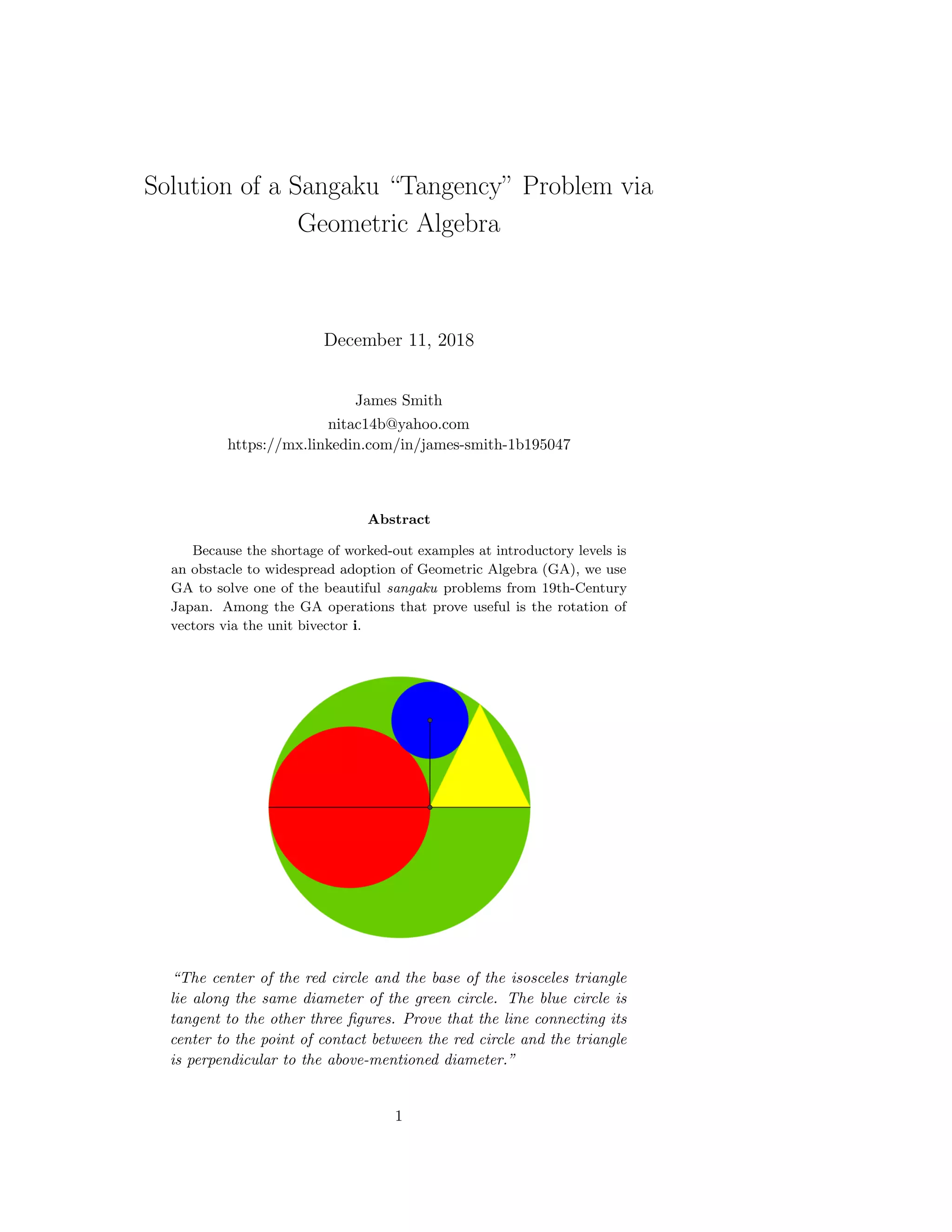
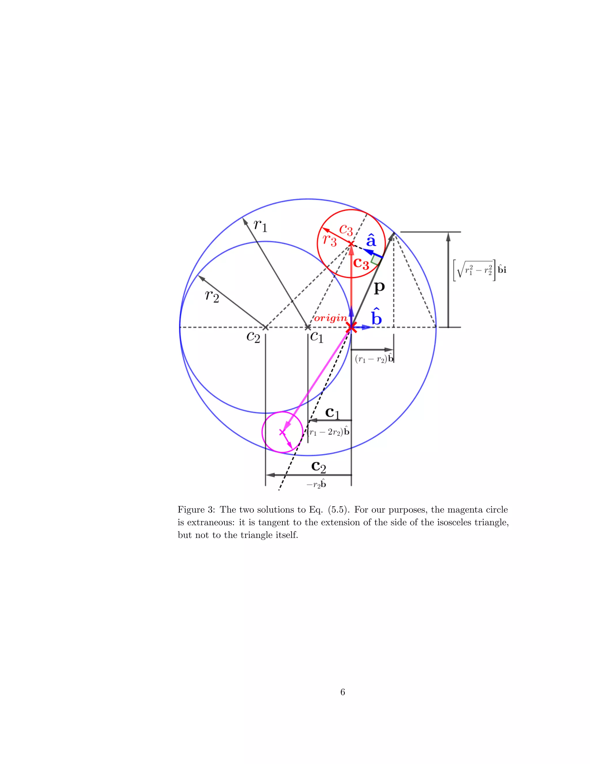
Download to read offline
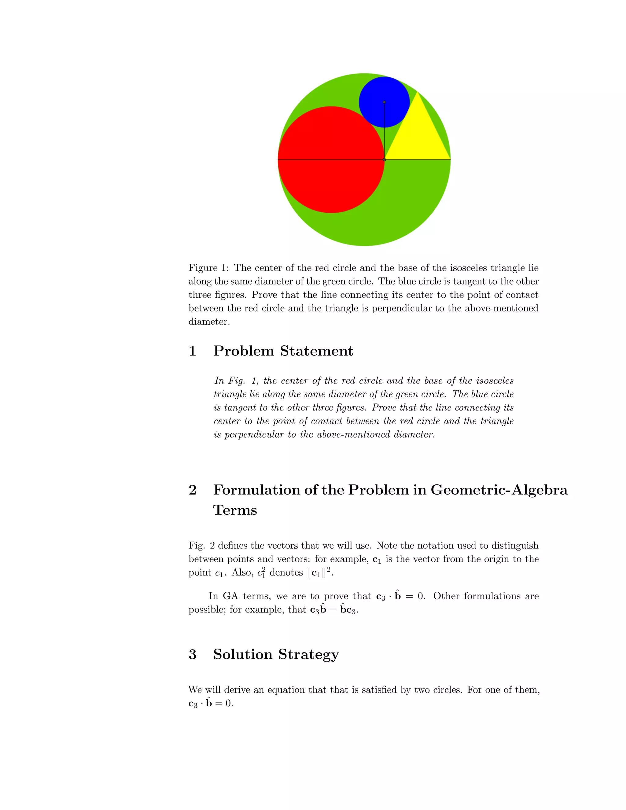

This document presents a solution to a tangency problem from a 19th-century Japanese sangaku using geometric algebra. The author derives necessary equations and proves that specified relationships between circles and lines hold under the conditions of the problem. Two solutions are identified, with one confirming the required tangency and the other deemed extraneous.


