SlideShare a Scribd company logo
1 of 54
Download to read offline
Learning Geometric Algebra by Modeling
Motions of the Earth and Shadows of Gnomons
to Predict Solar Azimuths and Altitudes
April 24, 2018
James Smith
nitac14b@yahoo.com
https://mx.linkedin.com/in/james-smith-1b195047
“Our first step in developing an expression for the orientation of
“our” gnomon: Diagramming its location at the instant of the 2016
December solstice.”
Abstract
Because the shortage of worked-out examples at introductory levels is
an obstacle to widespread adoption of Geometric Algebra (GA), we use
GA to calculate Solar azimuths and altitudes as a function of time via the
heliocentric model. We begin by representing the Earth’s motions in GA
terms. Our representation incorporates an estimate of the time at which the
Earth would have reached perihelion in 2017 if not affected by the Moon’s
gravity. Using the geometry of the December 2016 solstice as a starting
1
point, we then employ GA’s capacities for handling rotations to determine
the orientation of a gnomon at any given latitude and longitude during the
period between the December solstices of 2016 and 2017. Subsequently,
we derive equations for two angles: that between the Sun’s rays and the
gnomon’s shaft, and that between the gnomon’s shadow and the direction
“north” as traced on the ground at the gnomon’s location. To validate our
equations, we convert those angles to Solar azimuths and altitudes for
comparison with simulations made by the program Stellarium. As further
validation, we analyze our equations algebraically to predict (for example)
the precise timings and locations of sunrises, sunsets, and Solar zeniths on
the solstices and equinoxes. We emphasize that the accuracy of the results
is only to be expected, given the high accuracy of the heliocentric model
itself, and that the relevance of this work is the efficiency with which that
model can be implemented via GA for teaching at the introductory level.
On that point, comments and debate are encouraged and welcome.
2
Contents
1 Introduction 8
2 Review of Relevant Information about Kepler Orbits, Earth’s
orientation, and GA 10
2.1 The Gnomon and Its Uses . . . . . . . . . . . . . . . . . . . . . . 10
2.2 The Earth’s Kepler Orbit, and the Geometry of Solstices and
Equinoxes . . . . . . . . . . . . . . . . . . . . . . . . . . . . . . . 13
2.2.1 The Earth’s Kepler Orbit . . . . . . . . . . . . . . . . . . 13
2.2.2 Geometry of Solstices and Equinoxes . . . . . . . . . . . . 15
2.2.3 Summary of our Review of the Earth’s Orbit and the
Geometry of Equinoxes and Solstices . . . . . . . . . . . . 15
2.3 Review of GA . . . . . . . . . . . . . . . . . . . . . . . . . . . . . 17
2.3.1 Some General Comments on GA . . . . . . . . . . . . . . 18
2.3.2 Rotations and their Representations in GA . . . . . . . . 19
2.3.3 Angles Between Projected Vectors . . . . . . . . . . . . . 22
2.4 Observations on the Background . . . . . . . . . . . . . . . . . . 25
3 Detailed Formulation of Model in GA Terms 26
3.1 A Still-Unresolved Detail: How to Express ˆgL (t): The Orientation
of Our Gnomon as a Function of Time . . . . . . . . . . . . . . . 26
3.1.1 Finding an Idea . . . . . . . . . . . . . . . . . . . . . . . . 27
3.1.2 Expressing the Necessary Rotations via GA . . . . . . . . 28
3.1.3 Formulating the Bivectors Needed for the Rotations . . . 30
3.1.4 Celestial North: ˆnc . . . . . . . . . . . . . . . . . . . . . . 32
3.2 Our Model, in Words and in GA Terms . . . . . . . . . . . . . . 32
4 Derivations of Formulas 34
4.1 ˆr (t), ˆrs . . . . . . . . . . . . . . . . . . . . . . . . . . . . . . . . 35
4.2 ˆMs . . . . . . . . . . . . . . . . . . . . . . . . . . . . . . . . . . . 35
4.3 ˆnc . . . . . . . . . . . . . . . . . . . . . . . . . . . . . . . . . . . 36
4.4 ˆgsλ . . . . . . . . . . . . . . . . . . . . . . . . . . . . . . . . . . . 36
4.5 ˆQ . . . . . . . . . . . . . . . . . . . . . . . . . . . . . . . . . . . 37
4.6 Our Gnomon’s Direction . . . . . . . . . . . . . . . . . . . . . . . 37
4.7 The Angle α (t) . . . . . . . . . . . . . . . . . . . . . . . . . . . . 37
4.8 The Angle β (t) . . . . . . . . . . . . . . . . . . . . . . . . . . . . 38
4.8.1 Denominator of the sine and cosine of β (t) . . . . . . . . 38
4.8.2 Numerators of sin β (t) and cos β (t) . . . . . . . . . . . . 38
5 Validation of the Model and Calculations 39
5.0.1 Data for Earth’s Orbit, the December 2016 Solstice, Port
Moresby, and San Crist´obal de Las Casas . . . . . . . . . 39
5.1 Predictions, from Mathematical Analyses of Formulas, about
Solar Zeniths and the Sun’s Azimuths at Sunrise and Sunset . . 42
5.1.1 On the March Equinox: Sunrise, Sunset, and the Move-
ment of the Shadow’s Endpoint . . . . . . . . . . . . . . . 42
5.1.2 Azimuths of Sunrise and Sunset on the Solstices . . . . . 45
5.1.3 Solar Zeniths on the Solstices and Equinoxes . . . . . . . 47
5.2 Numerical Predictions of Sun’s Azimuth and Elevation as Seen
from Specific Locations at Specific Times . . . . . . . . . . . . . 49
5.3 Discussion of Results from the Validations . . . . . . . . . . . . . 50
6 Conclusions 50
List of Figures
1 Students using a gnomon at a school in India ([1]). . . . . . . . 9
2 Schematic diagram of the Sun, the gnomon, and the gnomon’s
shadow on the flat, horizontal surface surrounding the gnomon. . 11
3 Showing the angle α between the Sun’s rays and the shaft of the
gnomon. The angle of the Sun’s altitude (also called the angle of
elevation) is the complement of α. . . . . . . . . . . . . . . . . . 11
4
4 β is the angle of rotation from “Local North” (i.e., the direction
“geographic north” as traced on the ground at the observer’s
location) and the gnomon’s shadow. Later in this document, we
will define the counterclockwise sense of β as positive. . . . . . . 12
5 Relationship between β and the Sun’s azimuth. . . . . . . . . . . 12
6 Schematic of the Earth’s Kepler orbit, defining the elements φ, θ,
, and ˆr used in this analysis. The plane of the Earth’s orbit is
known as the ecliptic. (Reproduced from [7].) . . . . . . . . . . . 14
7 The position of the 2017 perihelion with respect to the December
2016 solstice. Red arrows show the direction in which the north
end of the Earth’s rotational axis points. The line connecting the
positions of the Earth at the equinoxes is not perfectly perpendic-
ular to the line connecting the positions at the solstices because
the Earth’s axis precesses by about 1/70
◦
per year. (Reproduced
from [7].) . . . . . . . . . . . . . . . . . . . . . . . . . . . . . . . 14
8 The relationship between the Sun, Earth, ecliptic, and the Earth’s
rotational axis. For our purposes, the orientation of the rotational
axis is constant during a given year, and the line connecting the
positions of the Earth at the equinoxes can be taken as perfectly
perpendicular to the line connecting the positions at the solstices.
(Reproduced from [7].) . . . . . . . . . . . . . . . . . . . . . . . . 15
9 Geometry of the equinoxes: the Earth’s axis of rotation lies within
the plane that is perpendicular to the ecliptic and to the line
connecting the centers of the Earth and Sun. (Reproduced from
[7].) . . . . . . . . . . . . . . . . . . . . . . . . . . . . . . . . . . 16
10 Geometry of the solstices: the Earth’s axis of rotation lies within
the plane that is perpendicular to the ecliptic, and which also
contains the line that connects the centers of the Earth and Sun.
(Reproduced from [7].) . . . . . . . . . . . . . . . . . . . . . . . . 16
11 One of the goals of our review: finding a convenient instant at
which a gnomon with a known location points in an identifiable
direction. At the instant of the December 2016 solstice, a gnomon
along the meridian that faces the Sun directly, and whose south
latitude is equal to the angle of inclination of the Earth’s rotational
axis with respect to the ecliptic plane, will point in the direction
−ˆr. . . . . . . . . . . . . . . . . . . . . . . . . . . . . . . . . . . . 17
12 Rotation of the vector w through the bivector angle ˆNγ, to
produce the vector w . . . . . . . . . . . . . . . . . . . . . . . . . 20
13 Rotation of bivector P by the bivector angle ˆNγ to give the
bivector H. . . . . . . . . . . . . . . . . . . . . . . . . . . . . . . 22
5
14 Reproduced from [12]. The flat, horizontal surface surrounding
the gnomon is a plane tangent to the Earth (assumed spherical)
at the point at which our gnomon is embedded . . . . . . . . . . 23
15 Reproduced from [12]. Note that the plane that contains the
Earth’s rotational axis and the meridian on which the gnomon is
located cuts the tangent plane along the direction that we have
been calling “local north”. Therefore, the direction “local north”
is the perpendicular projection of the direction of the Earth’s
rotational axis (labeled here as ˆnc) upon the flat, horizontal
surface on which our gnomon stands. . . . . . . . . . . . . . . . . 23
16 The problem treated in GA terms by [12]: the angle between
the projections of two vectors, u and v, upon a unit bivector ˆN
whose dual is ˆe. . . . . . . . . . . . . . . . . . . . . . . . . . . . 24
17 Our first step in developing an expression for the orientation of
“our” gnomon at any time: making a diagram of its location and
that of the solstice gnomon, in terms of their respective latitudes
and longitudes, at the instant of the 2016 December solstice (ts).
The solstice gnomon is that which points directly at the Sun at
that instant; thus, its orientation is −ˆrs. . . . . . . . . . . . . . . 27
18 The second step in developing an expression for the orientation of
our gnomon at any time: moving the solstice gnomon along the
solstice meridian to the latitude (λ) of our gnomon. The vector
of the gnomon in that position is ˆgsλ. . . . . . . . . . . . . . . . 28
19 The third step in developing an expression for the orientation of
“our” gnomon at any time: moving the ˆgsλ gnomon along latitude
λ longitude (µ) of our gnomon, whose orientation at the instant
of the 2016 December solstice is ˆg (ts). . . . . . . . . . . . . . . . 29
20 Schematic diagram of the Earth’s Kepler orbit, showing the vec-
tors ˆa and ˆb along with the unit bivector ˆC = ˆa ∧ ˆb = ˆaˆb .
The arrow next to the square representing ˆC shows ˆC’s positive
sense. Because that sense is in the direction of the Earth’s orbit,
ˆr (t) = ˆae
ˆCθ(t)
. . . . . . . . . . . . . . . . . . . . . . . . . . . . . 31
21 Definition of the vector ˆc that we will use in formulating ˆMs. The
set of vectors ˆa, ˆb, ˆc forms a right-handed, orthonormal basis. 31
22 Illustrating the use of ˆc, which is ˆC’s dual. The bivector (−ˆrs)∧ˆc
has the characteristics that we specified earlier for ˆMs. The arrow
next to the square representing ˆMs shows ˆMs’s positive sense. . 32
23 ˆQ is the rotation of ˆC through the bivector angle ˆMη. . . . . . . 34
6
24 The model, in GA terms. Arrows show the positive senses of
the bivectors ˆQ and ˆT. Vector ˆgL (t) rotates at constant angular
velocity ˆQω. The vector ˆr (t) varies with time according to the
Kepler equation ((2.1)). Vector ˆnc is the dual of ˆQ. Vector ˆgL (t)
is the dual of bivector ˆT (t). Not shown is the angle α between
−ˆgL (t) and ˆr (t). . . . . . . . . . . . . . . . . . . . . . . . . . . . 35
25 Relative positions of meridians of Port Moresby and San Crist´obal. 40
26 Because we measure latitudes from the equator, the latitudes λ
and π − λ are in fact the same latitude. . . . . . . . . . . . . . . 43
27 For simplicity, we’ve written the vector s (t) and the angles α (t)
and β (t) as s, α, and β. The length, s , of the shadow cast by
a gnomon of height g is g tan α. We wish to calculate the
length of s’s projection upon the direction “local north” on the
days of equinoxes. . . . . . . . . . . . . . . . . . . . . . . . . . . 45
28 On the day of an equinox, the trajectory of the end of the gnomon’s
shadow is a straight, east-west line at the distance g tan λ from
the base of the gnomon. . . . . . . . . . . . . . . . . . . . . . . . 46
List of Tables
1 Formulas for calculating azimuths according to the algebraic signs
of sin β and cos β. For example, if sin β < 0 and cos β ≥ 0, then
Azimuth = 180◦
+ arcsin | sin β| . . . . . . . . . . . . . . . . . . 11
2 Summary of the quantities in our model. . . . . . . . . . . . . . . 33
3 Summary of the parameters used in validating the model. ”Days”
are tropical days. The quantity “∆µ is µ − µs. . . . . . . . . . . 41
4 Times and dates of solstices and equinoxes for the year 2017, and
the number of tropical days between each event and the December
2016 solstice. (Adapted and corrected from [7].) . . . . . . . . . . 41
5 Comparison of Sun’s azimuths and altitudes according to atellar-
ium, to Those calculated from Eqs. (4.10), (4.11), (4.12), (4.13),
and (4.14), as seen from Port Moresby, Papua New Guinea on
three dates in 2017. All of the calculations are implemented in [16]. 51
6 Comparison of Sun’s azimuths and altitudes according to Stellar-
ium, to those calculated from Eqs. (4.10), (4.11), (4.12), (4.13),
and (4.14), as seen from San Crist´obal de Las Casas, Chiapas,
Mexico on three dates in 2017. All of the calculations are imple-
mented in [16]. . . . . . . . . . . . . . . . . . . . . . . . . . . . . 52
7
7 Solar azimuths and altitudes as seen from San Crist´obal de Las
Casas, according to Stellarium, at five-minute intervals around
UTC 4 October 2071 22:30:00 . . . . . . . . . . . . . . . . . . . . 52
1 Introduction
Geometric Algebra (GA) holds promise as a means for formulating and solving
problems in many different branches of mathematics and science. This document
contributes to addressing one of the obstacles to GA’s wider adoption: the
shortage of instructional materials that use GA to solve non-trivial problems
that are accessible to students who are in high school or the first year of university.
In this document, we’ll use GA for calculations that are related to gnomons
(Fig. 1) —astronomical instruments of a type that dates to antiquity. Many
simple, interesting experiments that use it are described in detail on line (e.g.
[2]), and can be performed by students to check predictions such as those which
we will make here. We will see, too, that through use of simple geometric and
trigonometric relations, inferences drawn from our gnomon equations can be
transformed into predictions that we can check via free planetarium software
such as Stellarium ([3]).
A key goal of this document is to make clear the relationship between
the skill of modeling physical systems, and the nature and capabilities of the
mathematical tools that are available to the modeler. The gnomon is a good
example for teaching that relationship because it shows the benefits of “seeing”
a system in terms of rotations—an operation to which GA is especially suited.
Toward that end, our specific goals will be
1. To use GA to predict the following for any location on Earth, at any time
between the December 2016 solstice and the December 2017 solstice:
(a) the angle between the Sun’s rays and the gnomon; and
(b) the angle between local north and the gnomon’s shadow.
2. To validate our model by comparing our predictions to results of simple
gnomon observations, and to simulations made by the planetarium program
Stellarium ([3]).
The same calculations may be done for other years using data available at [4].
This document begins by reviewing relevant information on Kepler orbits,
the geometry of the Earth’s orientation with respect to the plane of its orbit
about the Sun, and GA. Based upon that review, we’ll develop a model, then
derive the necessary equations. We’ll find that they are surprisingly amenable
to analyses that let us test key predictions without needing to do numerical
calculations. (Although we will of course do such calculations as well.)
8
Figure 1: Students using a gnomon at a school in India ([1]).
9
2 Review of Relevant Information about Kepler
Orbits, Earth’s orientation, and GA
“Our” gnomon. To get the most out of this review, we’ll want to keep the document’s goals
in mind. Let’s state them again, but this time we’ll refer to the gnomon for
which we want to calculate angles, etc. as simply “our gnomon”:
1. To use Geometric algebra to predict the following, at any time between
the December 2016 solstice and the December 2017 solstice:
(a) the angle between the Sun’s rays and our gnomon; and
(b) the angle between local north and our gnomon’s shadow.
2. To validate our model by comparing our predictions to results of simple
gnomon observations, and to simulations made by the planetarium program
Stellarium ([3]).
Given our goals, a reasonable thing to look for during our review is some
specific moment at which we can identify both of the following: the direction of
the Sun’s rays, and the direction in which our gnomon is pointing. Our goal
would then be to find a way to use that information to calculate, via GA, those
same directions for any other instant in time that might interest us.
2.1 The Gnomon and Its Uses
A gnomon is nothing more than a vertical stick, pole, or (in some cases) structure
surrounded by a flat, horizontal surface of appropriate size (Fig. 2). Over the
course of a year, the trajectory followed by the end of the gnomon’s shadow
changes systematically from one day to the next. Most notably, that trajectory
is an almost-perfect east-west line on the days of the equinoxes ([2]). Typical
experiments done with gnomons include tracing that trajectory for subsequent
mathematical analysis. Younger students enjoy measuring the angle β between
local north and the gnomon’s shadow, and the angle α between the gnomon and
a string stretched from the tip of the gnomon to the end of the shadow (Figs. 3
and 4).
Figs. 3 –5 and Table 1 show how to determine the Sun’s azimuth and
altitude from the angles α and β.
The shaft of the gnomon can be
regarded as an extension of the
line segment that runs from the
center of the Earth to the
gnomon’s base.
Please note something that will be important in our development of a model:
because the Earth’s deviation from perfect sphericity is less than 0.3% ([5]), the
shaft of the gnomon can be regraded as an extension of the line segment that
runs from the center of the Earth to the gnomon’s base.
10
Figure 2: Schematic diagram of the Sun, the gnomon, and the gnomon’s shadow
on the flat, horizontal surface surrounding the gnomon.
Figure 3: Showing the angle α between the Sun’s rays and the shaft of the
gnomon. The angle of the Sun’s altitude (also called the angle of elevation) is
the complement of α.
Table 1: Formulas for calculating azimuths according to the algebraic signs
of sin β and cos β. For example, if sin β < 0 and cos β ≥ 0, then Azimuth =
180◦
+ arcsin | sin β| .
sin β < 0 sin β ≥ 0
cos β < 0 360◦
− arcsin | sin β| arcsin | sin β|
cos β ≥ 0 180◦
+ arcsin | sin β| 180◦
− arcsin | sin β|
11
Figure 4: β is the angle of rotation from “Local North” (i.e., the direction
“geographic north” as traced on the ground at the observer’s location) and the
gnomon’s shadow. Later in this document, we will define the counterclockwise
sense of β as positive.
Figure 5: Geometrical bases for the formulas presented in Table 1 for determining
the Sun’s azimuth from sin β and cos β. Diagram is a schematic of an aerial
view of a plaza in which our gnomon is set. The Sun is in the part of the sky
opposite the shadow. Angle β is positive counter-clockwise from local north,
and the Sun’s azimuth is positive clockwise from local north.
12
2.2 The Earth’s Kepler Orbit, and the Geometry of Sol-
stices and Equinoxes
2.2.1 The Earth’s Kepler Orbit
Fig. 6 shows key elements that we will use later: the vector ˆr from the center
of the Sun to the center of the Earth; the angles θ and φ; and the vector a,
from the center of the orbit through the center of the Sun, to the position of the
Earth’s center at perihelion.
Hestenes ([6], pp. 204-219) used GA to arrive at the well-known Kepler
equation for planetary motion:
2πt
T
= φ − sin φ. (2.1)
where T is the planet’s orbital period, t is the time elapsed since the planet was
at its perihelion, and is the orbit’s eccentricity. The angle φ is in radians.
For any given time t, the corresponding angle θ (t) is determined by first
solving Eq. (2.1) for φ (t), after which the corresponding value of θ is found ([6],
p. 219) via the relationship
tan
θ
2
=
1 +
1 −
1/2
tan
φ
2
, (2.2)
from which
θ = 2 tan−1 1 +
1 −
1/2
tan
φ
2
. (2.3)
Ref. [7] notes that for works like the present, we must estimate what the
timing and position of the Earth’s perihelion would be if the Earth’s orbit were
a perfect Keplerian ellipse that is unperturbed by the gravity of other bodies,
especially the Moon. Using a best-fit method, [7] estimated that the perihelion
of 2017 occurred 12.93 days after the instant of the December 2016 solstice, and
that that solstice therefore occurred at angle θ of 0.2301 rad before perihelion
(Fig. 7).
Note that Fig. 7 shows the line connecting the positions of the Earth
at the equinoxes as being perpendicular the line connecting the positions at
the solstices. Actually, there is a very slight non-perpendicularity because the
Earth’s axis precesses by about 1/70
◦
per year. That precession also causes a
twenty-minute difference between the lengths of the Tropical year (the time
between successive December solstices) and the Sidereal year (the time needed
for the Earth to complete one revolution of its orbit, as measured against a fixed
frame of reference such as the stars). The effects of precession will require us to
be careful to use the Tropical year of 365.242 days in our calculations instead
of the Sidereal year of 365.256 days, but will otherwise be negligible for our
purposes. Differences between various types of year are discussed further in [8]
and [9].
13
Figure 6: Schematic of the Earth’s Kepler orbit, defining the elements φ, θ,
, and ˆr used in this analysis. The plane of the Earth’s orbit is known as the
ecliptic. (Reproduced from [7].)
Figure 7: The position of the 2017 perihelion with respect to the December 2016
solstice. Red arrows show the direction in which the north end of the Earth’s
rotational axis points. The line connecting the positions of the Earth at the
equinoxes is not perfectly perpendicular to the line connecting the positions
at the solstices because the Earth’s axis precesses by about 1/70
◦
per year.
(Reproduced from [7].)
14
Figure 8: The relationship between the Sun, Earth, ecliptic, and the Earth’s
rotational axis. For our purposes, the orientation of the rotational axis is constant
during a given year, and the line connecting the positions of the Earth at the
equinoxes can be taken as perfectly perpendicular to the line connecting the
positions at the solstices. (Reproduced from [7].)
2.2.2 Geometry of Solstices and Equinoxes
During a given year, we can treat
the orientation of the Earth’s
equatorial plane as invariant.
As shown in Fig. 8, the Earth’s rotational axis is inclined with respect to
the plane of the Earth’s orbit, or ecliptic. For our purposes the orientation of
the rotational axis is constant during a given year (Section 2.2.1). Therefore, we
can treat the orientation of the Earth’s equatorial plane as invariant.
In the common language, the terms “equinox and “solstice” refer to days,
but astronomers also use those terms to refer to precise instants as well. At the
instant of an equinox, the Earth’s axis of rotation lies within the plane that is
perpendicular to the ecliptic and to the line connecting the centers of the Earth
and Sun (Fig. 9). In contrast, at the instant of a solstice the axis lies within the
plane that is perpendicular to the ecliptic, and which also contains the line that
connects the centers of the Earth and Sun (Fig. 10).
Using ideas similar to those given in [10], we can identify the meridian of
longitude that faces the Sun directly at any given instant. The specific instant
that interests us is that of the December 2016 solstice.
2.2.3 Summary of our Review of the Earth’s Orbit and the Geome-
try of Equinoxes and Solstices
Before we began to review this material, we had decided that as we went through
each topic, we would look for some specific instant at which we could identify
both of the following: (a) the direction of the Sun’s rays, and (b) the direction
in which our gnomon would be pointing.
15
Figure 9: Geometry of the equinoxes: the Earth’s axis of rotation lies within
the plane that is perpendicular to the ecliptic and to the line connecting the
centers of the Earth and Sun. (Reproduced from [7].)
Figure 10: Geometry of the solstices: the Earth’s axis of rotation lies within the
plane that is perpendicular to the ecliptic, and which also contains the line that
connects the centers of the Earth and Sun. (Reproduced from [7].)
16
Figure 11: One of the goals of our review: finding a convenient instant at which
a gnomon with a known location points in an identifiable direction. At the
instant of the December 2016 solstice, a gnomon along the meridian that faces
the Sun directly, and whose south latitude is equal to the angle of inclination of
the Earth’s rotational axis with respect to the ecliptic plane, will point in the
direction −ˆr.
The 2016 December solstice would seem to be a good choice. Although we
don’t know the orientation of our own gnomon at that instant, we can identify
the location of a gnomon that points directly at the Sun at that instant: its
latitude is equal to that of the Earth’s inclination with respect to the ecliptic
(Fig. 11), and its longitude is that of the meridian that faces the Sun directly.
From that information, and the latitude and longitude of our own location, we
should be able to determine the orientation of our gnomon at the instant of the
2016 December solstice.
For our purposes, the Sun’s rays
that reach the Earth are parallel
to ˆr.
We should also note that for our purposes, the Sun’s rays that reach the
Earth are parallel to ˆr.
2.3 Review of GA
At the end of the previous section (2.2.3), we identified a combination of specific
gnomon location and instant in time with respect to which we should be able to
express the orientation of our own gnomon at any other instant t that might
interest us. Of course, we will also be able to calculate the vector ˆr for any
instant t via Eqs. (2.1) and (2.3). Now, we’ll review what we’ve learned about
GA so that we may learn how do the above via rotations, if practical.
17
2.3.1 Some General Comments on GA
As both a math tutor and a self-taught student, I am all too aware of the
confusion that students experience when trying to form an accurate mental
model of that which a classroom teacher or the author of a textbook is striving
to communicate through a combination of words, symbols, and diagrams. I hope
that the following observations might help, although they are not intended to
be either rigorous or complete.
A sometimes-helpful recognition is that GA, as it applies to problems like
the gnomon, is an attempt to capture geometric aspects of 3-D reality. The
mathematicians who developed GA found that they could express that reality
through concepts—of their own invention—which came to be known as vectors,
bivectors, and trivectors, and through carefully-defined mathematical operations
that are termed “products” of various sorts.
Of course this characterization of GA is vague, but the important points
are that GA is a human invention, and that the choices of which concepts and
operations were to be used in the attempt to formulate and solve geometrical
problems was made by human beings. Those same human beings defined the
properties of the concepts; for example, they decided that any two vectors of
identical length, direction, and orientation are equal, regardless of where they
are located in space. (Or perhaps to be more correct, “regardless of where their
endpoints are located in space”.) The originators of the concept of vectors did
not include “position” among the characteristics of vectors for a very simple
reason: there was no need to do so, and they saw no benefit in doing so.
Similar comments apply to bivectors: their only characteristics are magni-
tude (“area”, in 3-D geometry), orientation, and sense (algebraic sign). Devel-
opers of GA were able to accomplish their goals without including shape and
location among bivectors’ characteristics.
To accomplish our own, gnomon-related goals via GA, we need to express
the ecliptic plane in terms of a specific GA bivector (one to which the plane
is parallel). We also need to express the relation between that bivector and
the one that is used for the equatorial plane, and we need to express each of
these bivectors in terms of the basis bivectors of whatever reference system we
might find convenient. Rather than go into those important skills in detail here,
we’ll see how to put them into practice when we develop our gnomon model,
and when we derive formulas for calculating the angles α and β. Additional
examples can be found in [11] and [12].
One final note before we review the relevant GA information: in this
document, there are times when we will use the symbol for a given bivector (e.g.,
Q) to represent both the bivector itself (which is a GA object) and the plane to
which that bivector is parallel. Where the meaning of the symbol is not made
clear by context, we’ll state, explicitly, which meaning is intended.
18
In somewhat the same vein, we should mention that we may talk about
rotating a physical plane (such as the plane that contains the meridian of
longitude on which a gnomon stands) in terms of rotating the bivector that
represents it. Said meridian rotates with the Earth, so in that sense the meridian
does rotate. However, when we are using the term “plane” in its strict Euclidean
sense, a plane is a distinct set of points. Thus, the rotation of a plane produces a
different plane, not the same plane in a different orientation. Similar comments
apply to bivectors. Thus. as a the meridian rotates with the Earth, it goes into
and out of alignment with a succession of bivectors.
To put that differently, let’s use the symbol ˆM to denote the bivector that’s
parallel to the plane that contains a certain meridian. We see immediately that
the bivector that’s aligned with the plane at time t1 may be different from that
with which the meridian plane is aligned at some other time t2. Therefore, “the”
bivector with which the meridian is aligned is a function of time. We’ll write
that function as ˆM (t). Having done so, we recognize that although ˆM (t) is a
set of bivectors, each ˆM (τ) for any specific value τ of the time t is a specific,
individual bivector.
2.3.2 Rotations and their Representations in GA
Let’s recall that our purpose in this document is not only to calculate the angles
α and β, etc., but also to learn how to employ GA effectively for the formulation
and solution of certain types of problems. We expect, reasonably, that the
gnomon problem will be a good one for learning how to use GA for expressing
rotations, and also for determining angles between vectors. Refs. [11] and [12]
treat those topics in detail, but we will present only the most-relevant and
-important observations here.
Rotation of a vector by a bivector angle When describing an angle of
rotation in GA, we are often well advised—for sake of clarity—to write it as
the product of the angle’s scalar measure (in radians) and the bivector of the
plane of rotation. Following that practice, we would say that the rotation of
a vector w through the angle γ (measured in radians) with respect to a plane
that is parallel to the unit bivector ˆQ, is the rotation of w through the bivector
angle ˆNγ. (For example, see Fig. 12.) References [6] (pp. 280-286) and [13] (pp.
89-91) derive and explain the following formula for finding the new vector, w ,
that results from that rotation :
w = e− ˆNγ/2
[w] e
ˆNγ/2
Notation: R ˆNγ
(w)
. (2.4) Notation: R ˆNγ (w) is the
rotation of the vector w by the
bivector angle ˆNγ.
For our convenience later in this document, we will follow Reference [13] (p.
89) in saying that the factor e− ˆNγ/2
represents the rotation R ˆNγ. That factor
19
Figure 12: Rotation of the vector w through the bivector angle ˆNγ, to produce
the vector w .
is a quaternion, but in GA terms it is a multivector. We can see that from
the following identity, which holds for any unit bivector ˆB and any angle ξ
(measured in radians):
exp ˆBξ ≡ cos ξ + ˆB sin ξ.
The representation of a rotation.
Thus,
e− ˆNγ/2
= cos
γ
2
− ˆN sin
γ
2
. (2.5)
In our choice of symbols for
basis vectors and bivectors,
we´re following [13], p. 82.
In this document, we’ll restrict our treatment of rotations to three-dimensional
Geometric Algebra (G3
). In that algebra, and using a right-handed reference
system with orthonormal basis vectors ˆa, ˆb, and ˆc, we may express the unit
bivector ˆN as a linear combination of the basis bivectors ˆaˆb, ˆbˆc, and ˆaˆc :
ˆN = ˆaˆbnab + ˆbˆcnbc + ˆaˆcnac,
in which nab, nbc, and nac are scalars, and n2
ab + n2
bc + n2
ac = 1.
If we now write w as w = ˆawa + ˆbwb + ˆcwc, Eq. (2.4) becomes
w = cos
γ
2
− ˆN sin
γ
2
[w] cos
γ
2
+ ˆN sin
γ
2
= cos
γ
2
− ˆaˆbqc + ˆbˆcqa − ˆaˆcqb sin
γ
2
ˆawa + ˆbwb + ˆcwc cos
γ
2
+ ˆaˆbqc + ˆbˆcqa − ˆaˆcqb sin
γ
2
. (2.6)
Expanding the right-hand side of that result, we’d obtain 48 (!) terms, some of
which would simplify to scalar multiples of ˆa, ˆb, and ˆc, and others of which will
simplify to scalar multiples of the trivector ˆaˆbˆc. The latter terms would cancel,
leaving an expression for w in terms of ˆa, ˆb, and ˆc .
Now, we define four scalar variables:
20
• fo = cos
γ
2
;
• fab = nab sin
γ
2
;
• fbc = nbc sin
γ
2
; and
• fac = nac sin
γ
2
.
Using these variables, Eq. (2.6) becomes
w = fo − ˆaˆbfab + ˆbˆcfbc + ˆaˆcfac ˆawa + ˆbwb + ˆcwc fo + ˆaˆbfab + ˆbˆcfbc + ˆaˆcfac .
After expanding and simplifying the right-hand side, we obtain
w = ˆa wa f2
o − f2
ab + f2
bc − f2
ac + wb (-2fofab − 2fbcfac) + wc (-2fofac + 2fabfbc)
+ ˆb wa (2fofab − 2fbcfac) + wb f2
o − f2
ab − f2
bc + f2
ac + wc (-2fofbc − 2fabfac)
+ ˆc wa (2fofac + 2fabfbc) + wb (2fofbc − 2fabfac) + wc f2
o + f2
ab − f2
bc − f2
ac .
(2.7)
Note that in terms of our four scalar variables fo, fab, fbc, and fac, the
representation e− ˆNγ/2
of the rotation is
e− ˆNγ/2
= fo − ˆaˆbfab + ˆbˆcfbc + ˆaˆcfac . (2.8)
Because of the convenience with which Eq. (2.7) can be implemented, the
remainder of this document will express the representations of various rotations
of interest in the form of Eq. (2.8).
Rotation of a bivector Fig. 13 illustrates the rotation of a bivector P by
the bivector angle ˆNγ to give a new bivector, H. In his Theorem 7.5, Macdonald
([13], p. 125) states that if a blade P is rotated by the bivector angle ˆNγ, the
result will be the blade
R ˆNγ (P) = e− ˆNγ/2
[P] e
ˆNγ/2
. (2.9)
To express the result as a linear combination of the unit bivectors ˆaˆb, ˆbˆc,
and ˆaˆc, we begin by writing the unit bivector ˆN as ˆN = ˆaˆbnab + ˆbˆcnbc + ˆaˆcnac,
so that we may write the representation of the rotation in exactly the same way
as we did for the rotation of a vector:
e− ˆNγ/2
= fo − ˆaˆbfab + ˆbˆcfbc + ˆaˆcfac ,
with fo = cos
γ
2
; fab = nab sin
γ
2
; fbc = nbc sin
γ
2
; fac = nac sin
γ
2
.
Next, we write P as P = ˆaˆbpab + ˆbˆcpbc + ˆaˆcpac. Making these substitutions
in Eq. (2.9), then expanding and simplifying, we obtain
21
Figure 13: Rotation of bivector P by the bivector angle ˆNγ to give the bivector
H.
R ˆNγ (P) = ˆaˆb pab 1 − 2f2
bc − 2f2
ac
+2 [fab (fbcpbc + facpac) + fo (facpbc − fbcpac)]}
+ ˆbˆc pbc 1 − 2f2
ab − 2f2
ac
+2 [fbc (fabpab + facpac) + fo (fabpac − facpab)]}
+ ˆaˆc pac 1 − 2f2
ab − 2f2
bc
+2 [fac (fabpab + fbcpbc) + fo (fbcpab − fabpbc)]} .
(2.10)
2.3.3 Angles Between Projected Vectors
Ref. [12] treats this topics in detail, noting that the direction that we have been
calling “local north” is the perpendicular projection of the Earth’s rotational
axis upon a plane that is tangent to the Earth’s surface (assumed perfectly
spherical) at the gnomon’s location (Figs. 14 and 15).
Another observation in [12] is that the gnomon’s shadow is the the projection
of ˆr upon that same plane. Thus, our angle β is the angle between those two
projections. Ref. [12] considered precisely that sort of problem in GA terms:
the angle between the projections of two vectors, u and v, upon a unit bivector
ˆP whose dual is ˆe (Fig. 16). Writing these elements as
• u = ˆaua + ˆbub + ˆcuc,
22
Figure 14: Reproduced from [12]. The flat, horizontal surface surrounding the
gnomon is a plane tangent to the Earth (assumed spherical) at the point at
which our gnomon is embedded .
Figure 15: Reproduced from [12]. Note that the plane that contains the Earth’s
rotational axis and the meridian on which the gnomon is located cuts the tangent
plane along the direction that we have been calling “local north”. Therefore,
the direction “local north” is the perpendicular projection of the direction of
the Earth’s rotational axis (labeled here as ˆnc) upon the flat, horizontal surface
on which our gnomon stands.
23
Figure 16: The problem treated in GA terms by [12]: the angle between the
projections of two vectors, u and v, upon a unit bivector ˆN whose dual is ˆe.
• v = ˆava + ˆbvb + ˆcvc,
• e = ˆaea + ˆbeb + ˆcec, and
• ˆN = ˆaˆbnab + ˆbˆcnbc + ˆaˆcnac = ˆaˆbec + ˆbˆcea − ˆaˆceb ,
[12] found that
sin γ =
(uavb − ubva) nab + (ubvc − ucvb) nbc + (uavc − ucva) nac
u · ˆN v · ˆN
,
=
(uavb − ubva) ec + (ubvc − ucvb) ea − (uavc − ucva) eb
u · ˆN v · ˆN
, (2.11)
where u · ˆN and v · ˆN are the square roots of the expressions
u · ˆN 2
= u2
a 1 − e2
a + u2
b 1 − e2
b + u2
c 1 − e2
c
− 2uaubeaeb − 2ubucebec − 2uauceaec ,
(2.12a)
and
v · ˆN 2
= v2
a 1 − e2
a + v2
b 1 − e2
b + v2
c 1 − e2
c
− 2vavbeaeb − 2vbvcebec − 2vavceaec .
(2.12b)
24
Those expressions reduce to
u · ˆN 2
= u2
− (u · ˆe)
2
= u2
a + u2
b + u2
c − (uaea + ubeb + ucec)
2
,
(2.13a)
and
v · ˆN 2
= v2
− (v · ˆe)
2
= v2
a + v2
b + v2
c − (vaea + vbeb + vcec)
2
.
(2.13b)
Ref. [12] also found that
cos γ =
u · ˆN v · ˆN 0
u · ˆN v · ˆN
, (2.14)
where
u · ˆN v · ˆN 0 = uava 1 − n2
bc + ubvb 1 − n2
ac
+ ucvc 1 − n2
ab − (uavc + ucva) nabnbc
+ (ubvc + ucvb) nabnac + (uavb + ubva) nbcnac,
= uava 1 − e2
a + ubvb 1 − e2
b
+ ucvc 1 − e2
c − (uavc + ucva) eaec
− (ubvc + ucvb) ebec − (uavb + ubva) eaeb.
(2.15)
For our gnomon problem, the relevance of the above equations is that (1)
the unit vector that points from the center of the Earth to the tip of the gnomon
is also the dual of the bivector that is parallel to the plane on which the gnomon
is erected, and (2) the direction of the Sun’s rays is ˆr (Section 2.2.3).
2.4 Observations on the Background
Below, we’ll add the subscript L
to ˆg to denote the orientation of
“our” gnomon, and have used
ˆgL (t) instead of simply ˆgL in
recognition of the fact that the
orientation of the gnomon on a
rotating Earth is a function of
time.
One purpose of our review was to find a specific instant at which we could
identify both of the following: the direction of the Sun’s rays, and the direction
in which our gnomon is pointing. Fig. 11, showing the geometry of the 2016
December solstice, seems to provide a good starting point. We can now attempt
to use that information to calculate, via GA, the direction of the Sun’s rays and
our own gnomon at any other instant.
To express the following additional observations more conveniently, we’ll
denote the unit vector of the direction from the Earth’s center to the tip of our
25
gnomon as ˆgL (t), where t is the time elapsed since the Earth was at perihelion.
We’ll also note that ˆr, too, is a function of t, and write it as ˆr (t) . Similarly, α is
α (t), and β is β (t). Here, then, are the observations that might be most useful:
1. The key elements in our problem appear to be the direction of the Sun’s
rays; the ecliptic plane; the Earth’s axis of rotation; and the Earth’s
equatorial plane.
2. The ecliptic plane, equatorial plane, and direction of the Earth’s rotational
axis can all be taken as invariant.
3. So that we may use the Kepler equation and its various transformations,
we are well advised to define the time t as Kepler did. That is, t = 0 when
the Earth is at perihelion.
4. The direction of the Sun’s rays can be taken as ˆr (t).
5. From Figs. 3 and 11, we can deduce that cos α (t) = ˆr (t) · [−ˆgL (t)].
6. The direction “Local north” is the projection of the Earth’s rotational
axis upon the plane that is tangent to the Earth at the point at which our
gnomon is fixed. Because of the Earth’s rotation, local north is a function
of t.
7. The gnomon’s shadow is the projection of ˆr (t) upon that same plane.
8. To find the angle β (t), given ˆr (t) and ˆgL (t), we can use Eqs. (2.11) and
(2.14).
9. To find ˆr (t) at any given time, we can use Eqs. (2.1) and (2.2) .
Hence, we now have all we need for deriving formulas expressing angles
α and β for our gnomon at any time, if we can express the orientation of the
gnomon itself as a function of time.
3 Detailed Formulation of Model in GA Terms
3.1 A Still-Unresolved Detail: How to Express ˆgL (t): The
Orientation of Our Gnomon as a Function of Time
One of the purposes of this document is to show one way in which we might
puzzle through a problem like the gnomon, to arrive at a workable model and
solution strategy. Therefore, rather than just present a formula for ˆgL (t), we’ll
struggle with the problem a bit.
26
Figure 17: Our first step in developing an expression for the orientation of “our”
gnomon at any time: making a diagram of its location and that of the solstice
gnomon, in terms of their respective latitudes and longitudes, at the instant
of the 2016 December solstice (ts). The solstice gnomon is that which points
directly at the Sun at that instant; thus, its orientation is −ˆrs.
3.1.1 Finding an Idea
At this moment, our question is, “What do we want?” The answer is, “An
expression for ˆgL (t).”
So: what things did we note during our review, that might be useful? Here
are three possibilities:
• Via GA, we can formulate, readily, rotations about a given axis or by a
given bivector angle.
• The Earth rotates about its axis at a constant scalar angular velocity ω.
• We identified Fig. 11 as a promising starting-point for our present task.
An additional consideration might be that we should express the location
of “our” gnomon via its latitude λ and its longitude µ.
Thinking through the above observations. we might draft something like
Fig. 17, and conceive the follow overall plan:
1. First, we’ll derive an expression for the orientation of “our” gnomon at
the instant of the 2016 December solstice. We’ll denote that instant by ts.
Thus, the vector that gives the orientation of our gnomon at that instant
is ˆg (ts).
2. To find an expression for the orientation of our gnomon at any other time
t, we’ll rotate ˆg (ts) about the Earth’s axis via GA.
27
Figure 18: The second step in developing an expression for the orientation of our
gnomon at any time: moving the solstice gnomon along the solstice meridian to
the latitude (λ) of our gnomon. The vector of the gnomon in that position is
ˆgsλ.
We should make a note to
ourselves here, reminding us that
we’ll want to follow the usual
convention of expressing
northern latitudes as positive
angles, and southern latitudes as
negative ones.
Now, let’s flesh out that plan a bit. At this stage, we may alternate between
thinking in terms of “moving gnomons around on the globe” in Fig. 17, and
rotating the corresponding vectors. So: how can we identify ˆg (ts)? One way is
to recognize that we could do so by moving the solstice gnomon along meridians
of longitude and parallels of longitude to the position of our gnomon. Thus, we
would first slide the solstice gnomon along the solstice meridian, to the latitude
(λ) of our gnomon (Fig. 18). In GA terms, that movement is the rotation of the
vector −ˆrs through the scalar angle λ − (−η) , = λ + η. We’ll call the resulting
vector ˆgsλ, and identify the bivector for that rotation later.
Another note to ourselves: we’ll
follow the usual convention of
expressing eastern longitudes as
positive angles, and western
longitudes as negative ones.
Having “moved the solstice gnomon to our latitude”, and called the result
ˆgsλ, we’ll now slide ˆgsλ along our latitude until it stands on our meridian of
longitude, µ (Fig. 19). In GA terms, that movement is a rotation by the scalar
angle µ − µs about the Earth’s axis. The result will be the vector that we
called ˆg (ts): the orientation of our gnomon at the instant of the 2016 December
solstice.
Now, to find the orientation of our gnomon at any other instant, t, we just
rotate ˆg (ts) about the Earth’s axis by the angle ω (t − ts).
3.1.2 Expressing the Necessary Rotations via GA
How might we formulate in GA terms the rotations that we described in the
previous section? For the “sliding” along the solstice meridian, a reasonable
idea is to define a unit bivector ˆMs that’s parallel to the plane containing
that meridian, and whose positive sense is that of the rotation from −ˆrs to
28
Figure 19: The third step in developing an expression for the orientation of “our”
gnomon at any time: moving the ˆgsλ gnomon along latitude λ longitude (µ) of
our gnomon, whose orientation at the instant of the 2016 December solstice is
ˆg (ts).
ˆnc. Having defined ˆMs in this way, ˆgsλ is the rotation of −ˆrs through the
bivector angle ˆMs (λ + η). (That is, through the scalar multiple λ + η of the
unit bivector ˆMs.) The representation of that rotation ([13], p. 89) would then
be Z1 = e− ˆMs (λ + η) /2.
For the rotations about the Earth’s axis, we’ll define a unit vector ˆQ that’s
parallel to the equator. What should we choose as ˆQ’s positive sense? The
direction of the Earth’s rotation about its axis is a good choice, all the more
so because the dual of a ˆQ that’s so defined is none other than the vector
ˆnc. Using this definition of ˆQ, the representation of the rotation of ˆgsλ from
the solstice meridian to our own meridian to the longitude of our meridian at
time ts is Z2 = e− ˆQ (µ − µs) /2. The subsequent rotation of our meridian (and
thus of our gnomon) from the time ts to any other time t is represented by
Z3 = e− ˆQω (t − ts) /2.
Putting the preceding ideas together, we see that ˆgL (t) is the result of the
rotation of −ˆrs by the composite of the three above-described rotations. As
explained in [13], p. 125, the representation of that composite rotation is the
product Z3Z2Z1 of their respective rotations:
Z3Z2Z1 = e− ˆQω (t − ts) /2
e− ˆQ (µ − µs) /2
e− ˆMs (λ + η) /2
= e− ˆQ [µ − µs + ω (t − ts)] /2
e− ˆMs (λ + η) /2
.
To make that result more convenient, we’ll define k (µ, t) = µ − µs + ω (t − ts),
giving
Z3Z2Z1 = e− ˆQk (µ, t) /2
e− ˆMs (λ + η) /2
Because that result is the representation of the rotation that produces ˆgL (t)
29
from −ˆrs,
ˆgL (t) = e− ˆQk (µ, t) /2
e− ˆMs (λ + η) /2
[−ˆrs] e
ˆMs (λ + η) /2
e
ˆQk (µ, t) /2
The above having been said, we’re under no obligation to calculate ˆgL (t)
directly from ˆrs. Depending upon the complexity of the expressions that arise
when we make substitutions for ˆrs, ˆMs, and ˆQ, we might instead choose to first
derive an expression for ˆgsλ from ˆrs,
ˆgsλ = e− ˆMs (λ + η) /2
[−ˆrs] e
ˆMs (λ + η) /2
, (3.1)
after which we would calculate ˆgL (t) via
ˆgL (t) = e− ˆQk (µ, t) /2
[ˆgsλ] e
ˆQk (µ, t) /2
. (3.2)
Other reasons for choosing this route include the possibility of gaining greater
insight into the relationships between the calculations and the physical phenom-
ena, and the desire to check the results of each step to make sure that they make
sense.
3.1.3 Formulating the Bivectors Needed for the Rotations
In the previous section, we used GA’s capacities for formulating rotations to
express ˆgL (t) in terms of the vector ˆrs (= ˆr (ts)) and the time-invariant bivectors
ˆMs and ˆQ. Now, let’s develop expressions for those bivectors in terms of the
vectors ˆa and ˆb of the Earth’s Kepler orbit. Our purpose in doing so is to
facilitate the numerical calculations of α (t) and β (t) that we will wish to make.
ˆa ∧ ˆb = ˆaˆb because ˆa ⊥ ˆb. In Fig. 20, we introduce the unit bivector ˆC = ˆa ∧ ˆb = ˆaˆb . It’s parallel
to the ecliptic plane, and its positive sense is in the direction of the Earth’s
orbit. Thus, for any time t,
ˆr (t) = e− ˆCθ(t)/2
[ˆa] e
ˆCθ(t)/2
= ˆae
ˆCθ(t)
, (3.3)
because ˆa is parallel to ˆC. In particular, ˆrs = ˆae
ˆCθs
.
We decided in the previous section to define ˆMs as the unit bivector that is
parallel to the solstice meridian, and whose positive sense is in the direction of the
rotation from −ˆrs ˆnc . Examining Figs. 21–22, we see that those characteristics
are possessed by the bivector (−ˆrs) ∧ ˆc, where ˆc is ˆC’s dual. Comparing Figs.
20 and 22, we also see that the set of vectors ˆa, ˆb, ˆc forms a right-handed,
orthonormal basis—quite a favorable development for our purposes. Thus, we
define
ˆMs = (−ˆrs) ∧ ˆc
= −ˆrsˆc, (3.4)
30
Figure 20: Schematic diagram of the Earth’s Kepler orbit, showing the vectors
ˆa and ˆb along with the unit bivector ˆC = ˆa ∧ ˆb = ˆaˆb . The arrow next to
the square representing ˆC shows ˆC’s positive sense. Because that sense is in the
direction of the Earth’s orbit, ˆr (t) = ˆae
ˆCθ(t)
.
Figure 21: Definition of the vector ˆc that we will use in formulating ˆMs. The
set of vectors ˆa, ˆb, ˆc forms a right-handed, orthonormal basis.
31
Figure 22: Illustrating the use of ˆc, which is ˆC’s dual. The bivector (−ˆrs) ∧ ˆc
has the characteristics that we specified earlier for ˆMs. The arrow next to the
square representing ˆMs shows ˆMs’s positive sense.
because ˆrs ⊥ ˆc.
With ˆMs defined in this way, ˆQ, which we need for rotations about the
Earth’s axis, is just the rotation of ˆC through the bivector angle ˆMη Fig. 23:
ˆQ = e− ˆMsη/2 ˆC e
ˆMsη/2
. (3.5)
3.1.4 Celestial North: ˆnc
From Fig. 23, we can see that the rotation from ˆc to ˆnc is the same as that from
ˆMs to ˆQ. Therefore, having formulated ˆMs, we can now express ˆnc readily as
the rotation of ˆc by the bivector angle ˆMsη:
ˆnc = e− ˆMsη/2
[ˆc] e
ˆMsη/2
. (3.6)
We could also formulate it as dual of ˆQ.
3.2 Our Model, in Words and in GA Terms
We developed our model and defined its variables in the course of “puzzling-
through” the gnomon problem, so we should take time now to summarize and
organize (Table 2 ) before moving on to derive equations for the angles α and β.
32
Table 2: Summary of the quantities in our model.
Symbol Description
ˆa, ˆb, ˆc The right-handed, orthonormal basis of our reference system.
t Time, per Kepler equation. When t = 0, Earth is at perihelion.
ts Value of t at the instant of the 2016 December solstice.
η The angle of the equator with respect to the ecliptic. Positive if
in the positive sense of ˆMs.
λ Our (that is, our gnomon’s) latitude. Positive in the Northern
Hemisphere, negative in the Southern Hemisphere.
µ Our longitude, with East longitudes taken as positive.
µs Value of µ for the “solstice meridian”: that which faced the Sun
directly at the December 2016 solstice.
ω Angular velocity of the Earth’s rotation about its own axis.
k (µ, t) = µ − µs + ω (t − ts).
r (t) Vector from Sun’s center to Earth’s center at time t. Direction
of Sun’s rays is approximated as equal to ˆr (t).
ˆrs = ˆr (ts).
θ (t) Angle from ˆa to ˆr (t). Positive in the direction of the Earth’s
orbit, and thus if in the positive sense of ˆC.
θs = θ (ts) .
ˆC Unit bivector = ˆaˆb of the ecliptic plane. Assumed constant.
ˆMs Unit bivector of the solstice meridian. Equal to −ˆrsˆc.
ˆQ Unit bivector of Earth’s equatorial plane. Assumed constant;
equal to rotation of ˆQ by ˆMsη
ˆnc “Celestial North”: the direction from the center of the Earth to
the Geographic North Pole.
ˆnL (t) “Local north”: the direction, at t, of “north” at our location.
ˆgsλ Direction, at time ts, of a gnomon at latitude λ, longitude µs.
ˆgL (t) Direction, t, from base of our gnomon to its tip. This vector is
ˆT (t)’s dual.
ˆT (t) Unit bivector parallel to the plane that, at time t, is tangent to
Earth’s surface at base of our gnomon. ˆT (t)’s dual is ˆgL (t).
ˆs (t) Direction, at time t, from base of our gnomon to tip of its
shadow.
α (t) Angle between gnomon’s shaft and Sun’s rays at instant t.
β (t) Angle of rotation from ˆnL (t) to ˆs (t).
33
Figure 23: ˆQ is the rotation of ˆC through the bivector angle ˆMη.
Our model is that the Earth is perfectly spherical, and orbits the Sun
according to the Kepler model. The direction of the Sun’s rays is the same as
the direction ˆr (t) from the center of the Sun to the center of the Earth. The
Earth’s equatorial plane is inclined by angle η (assumed constant) with respect
to the ecliptic. The Earth rotates at constant angular velocity ω. At the instant
of the 2016 December solstice, the longitude that faces the Sun directly is µs.
Our gnomon is located at latitude λ, longitude µ, and casts a shadow upon a
plane that is tangent to the Earth at that same location.
We wish to be able to calculate, for any time t, the angle between the Sun’s
rays and the gnomon, and the angle between the direction “local north” and
the gnomon’s shadow.
In GA terms (Fig. 24), vector ˆgL (t) rotates at constant angular velocity
ˆQω. The vector ˆr (t) varies with time according to the Kepler equation ((2.1)).
Vector ˆnc is the dual of ˆQ. Vector ˆgL (t) is the dual of bivector ˆT (t).
We wish to be able to calculate, for any time t, (1) the angle between the
vectors ˆgL (t) and ˆr (t), and (2) the angle of rotation from ˆnc’s projection upon
ˆT (t) to ˆr (t)’s projection upon ˆT (t).
4 Derivations of Formulas
Several of the derivations use formulas that are developed in Section 2.3.2, and
implemented in Maxima in [14].
34
Figure 24: The model, in GA terms. Arrows show the positive senses of the
bivectors ˆQ and ˆT. Vector ˆgL (t) rotates at constant angular velocity ˆQω. The
vector ˆr (t) varies with time according to the Kepler equation ((2.1)). Vector ˆnc
is the dual of ˆQ. Vector ˆgL (t) is the dual of bivector ˆT (t). Not shown is the
angle α between −ˆgL (t) and ˆr (t).
4.1 ˆr (t), ˆrs
This vector is the rotation of ˆa through the bivector angle ˆCθ (t). Thus (Eq.
(3.3)),
ˆr (t) = ae
ˆCθ(t)
= ˆaeˆaˆbθ(t)
= ˆa cos θ (t) + ˆaˆb sin θ (t)
= ˆa cos θ (t) + ˆb sin θ (t) . (4.1)
Specifically,
ˆrs = ˆr (ts) = ˆa cos θs + ˆb sin θs. (4.2)
4.2 ˆMs
From Eq. (3.4), ˆMs = −ˆrsˆc. Thus, using the expression for −ˆrs from Eq. (4.2),
ˆMs = − ˆa cos θs + ˆb sin θs ˆc
= −ˆbˆc sin θs − ˆaˆc cos θs. (4.3)
35
ˆMs is also the rotation of the bivector ˆcˆa through the bivector angle ˆQθs:
ˆMs = e
−C
θs
2 [ˆcˆa] e
C
θs
2
= cos θs
2
− ˆaˆb sin θs
2
[ˆcˆa] cos θs
2
+ ˆaˆb sin θs
2
= −ˆbˆc sin θs − ˆaˆc cos θs.
4.3 ˆnc
This vector is the rotation of ˆc by the bivector angle ˆMsη. We’ll calculate ˆnc
using Eqs. (2.7) and (2.8). To do so, we need to write the representation of the
rotation by ˆMsη in the form fo − ˆaˆbfab + ˆbˆcfbc + ˆaˆcfac :
e
− ˆMs
η
2 = cos η
2
− −ˆbˆc sin θs − ˆaˆc cos θs sin η
2
= cos η
2
− ˆbˆc sin θs sin η
2
− ˆaˆc cos θs sin η
2
, (4.4)
so fo = cos η
2
, fab = 0, fbc = − sin θs sin η
2
, and fac = − cos θs sin η
2
. Therefore,
ˆnc = ˆa sin(η) cos θs
+ ˆb sin(η) sin θs
+ ˆc cos(η).
(4.5)
4.4 ˆgsλ
The vector ˆgsλ is the rotation of −ˆrs by the bivector angle ˆMs (η + λ). As was
the case for calculating ˆnc, we need to write the representation of our rotation
in the form fo − ˆaˆbfab + ˆbˆcfbc + ˆaˆcfac :
e
− ˆMs
η + λ
2 = cos η + λ
2
− −ˆbˆc sin θs − ˆaˆc cos θs sin η + λ
2
= cos η + λ
2
− ˆbˆc sin θs sin η + λ
2
− ˆaˆc cos θs sin η + λ
2
, (4.6)
so fo = cos η + λ
2
, fab = 0, fbc = − sin θs sin η + λ
2
, and fac = − cos θs sin η + λ
2
.
Therefore,
ˆgsλ = ˆa [− cos θs cos (η + λ)]
+ ˆb [− sin θs cos (η + λ)]
+ ˆc [sin (η + λ)] .
(4.7)
36
4.5 ˆQ
ˆQ is ˆC rotated through the bivector angle ˆMsη:
ˆQ = e
− ˆMs
η
2 ˆC e
ˆMs
η
2
= cos η
2
− −ˆbˆc sin θs − ˆaˆc cos θs sin η
2
ˆaˆb cos η
2
+ −ˆbˆc sin θs − ˆaˆc cos θs sin η
2
= ˆaˆb cos η + ˆbˆc cos θs sin η − ˆaˆc sin θs sin η. (4.8)
4.6 Our Gnomon’s Direction: ˆgL (t)
This vector is the rotation of ˆgsλ by the bivector angle ˆQk (µ, t). The pa-
rameters of our rotation are f0 = cos
k (µ, t)
2
, fab = cos η sin
k (µ, t)
2
, fbc =
cos θs sin(η) sin
k (µ, t)
2
, fac = − sin θs sin(η) sin
k (µ, t)
2
. Therefore, from Eqs.
(2.7) and (2.8),
ˆgL (t) = ˆa {sin θs cos λ sin k (µ, t) − cos θs cos (η + λ) + cos θs cos η cos λ [1 − cos k (µ, t)]}
+ˆb {sin θs cos η cos λ [1 − cos k (µ, t)] − sin θs cos (η + λ) − cos θs cos λ sin k (µ, t)}
+ˆc {sin (η + λ) − sin η cos λ [1 − cos k (µ, t)]}.
(4.9)
4.7 The Angle α (t)
As noted in Section 2.4, α (t) is the angle of rotation from -ˆgL (t) to ˆr (t). A
gnomon is a device for producing shadows, which occur only when the Sun is
above the horizon; in other words, when the inner product of -ˆgL (t) · ˆr (t) is
positive. Having ensured that, the only characteristic of α (t) that interests us is
its magnitude. Therefore, all we need to know is α (t)’s cosine, which is equal to
the inner product ˆu · ˆv. Therefore, cos α (t) = [-ˆgL (t)] · ˆr (t). We’ve developed
expressions for these two vectors (Eqs. (4.9) and (4.1), we find that
cos α = {cos (η + λ) − cos η cos λ [1 − cos k (µ, t)]} cos (θt − θs)
+ cos λ sin (θt − θs) sin k (µ, t) .
(4.10)
Some comments upon that equation: At the instant ts of the December
solstice, θ (t) = θs. In addition, for points along the meridian that’s aligned with
the Sun at that time (e.g., points along Ms), k (µ, t) = 0. Therefore, along that
meridian and at that instant, Eq. (4.10) reduces to cos α (ts) = cos (η + λ).
Does our answer make sense?Does that result make sense?
37
4.8 The Angle β (t)
We will find β (t) from its sine and cosine, which we will calculate according to
Section 2.3.3.
4.8.1 Denominator of the sine and cosine of β (t)
This denominator is the product of ˆnc · ˆT (t) and [ˆr (t)] · ˆT (t) . We’ll
treat each of those quantities in turn.
The norm ˆnc · ˆT (t) . To calculate this norm, we will use Eq. (2.12),
which expresses the norm of a vector’s projection upon a bivector in terms of
that bivector’s dual. In our case, the dual of ˆT (t) is ˆgL (t) (Eq. (4.9)), and
ˆnc is given by Eq. (4.3). The result, as given in [14], is ˆnc · ˆT (t) = |cos λ|.
However, |cos λ| = cos λ in our model because −π/2 ≤ λ ≤ π/2 . Thus,
ˆnc · ˆT (t) = cos λ. (4.11)
Does our answer make sense? A surprisingly simple result. Does it make sense? Let’s look at Fig. 14. We
can deduce that the angle between ˆnc and ˆT (t) is either λ or 180◦
+ λ. Because
ˆnc is a unit vector, the magnitude of RˆT (ˆnc) (i.e., of ˆnc’s projection upon ˆT (t))
is indeed cos λ. As explained in [12], ˆnc · ˆT (t) evaluates to a vector that is a
90◦
rotation of RˆT ( ˆnc), with no change in the latter’s magnitude. Therefore,
ˆnc · ˆT (t) = RˆT (ˆnc) = cos λ.
The norm [ˆr (t)] · ˆT (t) As shown in [14], using (4.1)’s expression for ˆr (t)
in Eq. (2.12) yields a result that I was not able to reduce to a simple form. Nor
was I able to do so by starting from the observation that because ˆr (t) is a unit
vector,
[ˆr (t)] · ˆT (t) 2
= 1 − {[ˆr (t)] · [ˆgL (t)]}
2
,
Does our answer make sense?
What should [ˆr (t)] · ˆT (t) be
when t = ts? Note that when
t = ts, θt = θs and k (µ, t) = 0.
from which ( [14])
[ˆr (t)] · ˆT (t) 2
= 1 − {[cos η cos λ (1 − cos k (µ, t)) − cos (η + λ)] cos [θt − θs]
− cos λ sin k (µ, t) sin [θ (t) − θs]}
2
.
(4.12)
4.8.2 Numerators of sin β (t) and cos β (t)
Eqs. (4.5), (4.1), and (4.9) (respectively) present the expressions that we
developed for ˆnc, ˆr (t), and ˆgL (t). To calculate the numerators of sin β (t) and
cos β (t), we will substitute those expressions for (respectively)u, v, and ˆe in
Eqs. (2.11) and (2.14). Those equations are implemented in [14], which is the
source from which we cite the results presented in the paragraphs that follow.
38
Note that cos λ (which is ˆnc · ˆT (t) , Eq. (4.11)) is a factor of every term
in both numerators.
Numerator of sin β (t) As given in [12], the numerator of sin β (t) is
Numerator of sin β (t) = cos λ cos k (µ, t) sin [θ (t) − θs]
− cos η cos λ sin k (µ, t) cos [θ (t) − θs] .
(4.13)
Numerator of cos β (t) As given in [12], the numerator of sin β is
Numerator of cos β (t) = cos λ sin λ sin k (µ, t) sin [θ (t) − θs]
+ cos η cos λ sin λ cos k (µ, t) cos [θ (t) − θs]
+ sin η cos2
λ cos [θ (t) − θs] .
(4.14)
5 Validation of the Model and Calculations
We’ll validate the model and calculations in two ways: (1) by deducing, from
mathematical analyses of our equations for α (t) and β (t), the latitudes at which
solar zeniths occur on the equinoxes and solstices, and the azimuths at which
the Sun sets on those dates; and (2) by making numerical predictions of the
Sun’s azimuth and altitude as seen at specific times from Port Moresby, Papua
New Guinea, and from San Crist´obal de Las Casas, Chiapas, Mexico.
Those locations were chosen because they lie on opposite sides of the equator,
and also on opposite sides of the meridian that faces the Sun at the instant of
the December 2016 solstice. Thus, their values of λ and µ − µs are of opposite
algebraic signs (Fig. 25). For that reason, they provide a way of detecting sign
errors in our calculations. Because the two cities also lie within the Tropics of
their respective hemispheres, the Sun will be in the northern half of the sky
during one part of the year, and in the southern half during the other. That
characteristic will enable us to detect other types of errors, if present.
5.0.1 Data for Earth’s Orbit, the December 2016 Solstice, Port
Moresby, and San Crist´obal de Las Casas
The Earth and its orbit Reference [5] gives the orbit’s eccentricity ( ) as
0.1671022, and its orbital period, T, 365.242 tropical days.
The inclination of the Earth’s rotational axis is 23.44◦
. At the December
solstice, the axis is pointed away from the Sun, so the algebraic sign of that angle
is positive. Thus, η = 23.44◦
. Identifying the Earth’s rotational angular velocity,
ω, requires some thought. As noted in [8], the Earth rotates by slightly more
than 360◦
during one tropical day. Over the course of a full year, that slight
39
Figure 25: Relative positions of the meridians of Port Moresby and San Crist´obal
de Las Casas with respect to the Greenwich Meridian and the meridian that
faces the Sun directly at the instant of the December 2016 solstice. Note that
∆µ = µ − µs.
daily excess adds up to one full rotation. Therefore, the Earth makes 366.242
rotations of 2π radians each in 365.242 tropical days, from which ω = 6.3004
radians/tropical day.
The December 2016 solstice Reference [7] found that for the December 2016
solstice, which occurred at UTC 21 December 2016 10:44:44, θs = −0.230099
radians, and ts = −12.9379 tropical days. Using the planetarium program
Stellarium ([3]), I found that the meridian of longitude that faced the Sun
directly at the instant of the solstice was E 18◦
33 (-0.32376 radians, according
to the sign convention used in our model): approximately that of Stockholm,
Sweden and Cape Town, Republic of South Africa.
Port Moresby and San Crist´obal de Las Casas According to [3], Port
Moresby’s latitude and longitude are S9◦
26 35.30 E147◦
10 46.98 , while San
Crist´obal’s are N16◦
44 12.00 W92◦
38 18.01 . Therefore, Port Moresby’s value
of µ − µs is +128◦
37 , or 2.2450 radians, and San Crist´obal´s is -1.9406 radians.
Summary of the parameters used in validating the model Tables 3
and 4 summarize the relevant data.
40
Table 3: Summary of the parameters used in validating the model. ”Days” are
tropical days. The quantity “∆µ is µ − µs.
Parameters of the Earth and its orbit
T, days η, radians ω, radians/day
0.16710 365.242 0.40911 6.30039
Parameters of the December 2016 solstice
Date (UTC) θs, radians ts, days µs, radians
21/12/2016
10:44:00
-0.23010 -12.938 0.32376
Parameters of Port Moresby and San Crist´obal de Las Casas
λ, radians ∆µ, radians
Port
Moresby
-0.16481 2.2450
San
Crist´obal
0.29211 -1.9406
Table 4: Times and dates of solstices and equinoxes for the year 2017, and the
number of tropical days between each event and the December 2016 solstice.
(Adapted and corrected from [7].)
Event UTC Time and date ([4]) t − ts, days
Dec. 2016 solst 21/12/2016 10:44:00 0.000
Mar. 2017 equin 20/03/2017 10:29:00 88.987
June 2017 solst 21/06/2017 04:24:00 181.736
Sept. 2017 equin 22/09/2017 20:02:00 275.388
Dec. 2017 solst 21/12/2017 16:28:00 365.239
41
5.1 Predictions, from Mathematical Analyses of Formu-
las, about Solar Zeniths and the Sun’s Azimuths at
Sunrise and Sunset
For convenience, we’ll repeat Eqs. (4.10), (4.13), and (4.14) here:
cos α (t) = {cos (η + λ) − cos η cos λ [1 − cos k (µ, t)]} cos (θt − θs)
+ cos λ sin (θt − θs) sin k (µ, t)
(5.1)
Numerator of sin β (t) = cos λ cos k (µ, t) sin [θ (t) − θs]
− cos η cos λ sin k (µ, t) cos [θ (t) − θs] .
(5.2)
Numerator of cos β (t) = cos λ sin λ sin k (µ, t) sin [θ (t) − θs]
+ cos η cos λ sin λ cos k (µ, t) cos [θ (t) − θs]
+ sin η cos2
λ cos [θ (t) − θs] .
(5.3)
We’ll also recall that from Eqs. (4.11) and (4.12), the denominator of sin β
and cos β is the product of cos λ and the square root of
1 − {[cos η cos λ (1 − cos k (µ, t)) − cos (η + λ)] cos [θt − θs]
− cos λ sin k (µ, t) sin [θ (t) − θs]}
2
.
(5.4)
Now, we’ll analyze those formulas to find out what they predict for the
azimuths and latitudes of sunrises, sunsets, and solar zeniths. In some cases,
we’ll also find it useful to recognize that because we measure latitudes from the
equator, the latitudes λ and π − λ are in fact the same latitude (Fig. 26).
5.1.1 On the March Equinox: Sunrise, Sunset, and the Movement
of the Shadow’s Endpoint
The two key ideas in these analyses are that the Sun’s rays are parallel to the
Earth’s surface at sunrise and sunset (thereforecos α = 0), and that at the instant
of the March equinox, θ (t) − θs = π/2. Combining those two observations, we
can deduce from Eq. (5.1) that at the instant of the March equinox sunrise,
cos λ sin k (µ, t) = 0. Thus, we have only two possibilities: either cos λ = 0, or
sin k (µ, t) = 0. The condition cos λ = 0 would mean that at the instant of an
equinox, sunset is occurring only at the north and south poles. We reject that
possibility, because we know that sunsets are never experienced at only one single,
precise latitude. Thus, we conclude that sin k (µ, t) = 0, and cos k (µ, t) = ±1.
42
Figure 26: Because we measure latitudes from the equator, the latitudes λ and
π − λ are in fact the same latitude.
The azimuth at which the Sun rises and sets on the equinoxes Sub-
stituting sin k (µ, t) = 0 and θ (t) − θs = π/2 in Eq. (5.4), we find that the
denominator of sin β is cos λ. Next, substituting sin k (µ, t) = 0, θ (t)−θs = π/2,
and cos k (µ, t) = ±1 in Eq. (5.2), the numerator of sin β is ± cos λ. Thus,
sin β = ±1.
What is the physical interpretation of that result? Let’s go back and
re-examine the condition sin k (µ, t) = 0. That condition is met by either of
k (µ, t) = 0 or k (µ, t) = π . Recalling that k (µ, t) = µ − µs + ω (t − ts),
we can now see that the condition sin k (µ, t) = 0 obtains at two longitudes:
µ = µs − ω (t − ts) and µ = π + [µs − ω (t − ts)]. The µ values of our two
longitudes differ by π. One inference from that result is that the two longitudes
are on opposite sides of the Earth. Another (from basic trig identities) is that
signs of those longitudes’ respective values of cos k (µ, t) are opposite in algebraic
sign. Therefore, of the two longitudes at which cos α = 0 at the instant of the
March equinox, cos k (µ, t) must be +1 for one of those longitudes, and −1 for
the other.
Following through on that result, the numerators of sin βfor those longitudes
are + cos λ and − cos λ, respectively, making their respective values of sin β +1
and −1. Thus, one of those longitudes is experiencing sunrise, and the other is
experiencing sunset.
The preceding analysis shows that for those two longitudes, cos λ sin k (µ, t) =
0, regardless of latitude at the instant of the March equinox. That is, all latitudes
are experiencing sunrise on one of those longitudes, and all latitudes are experi-
encing sunset on the other. Similar reasoning leads to the same conclusion for
43
the September equinox. This finding is familiar to anyone who drives eastward
to work around daybreak on the equinoxes: the Sun will be almost directly in
your eyes when on the drive to work in the morning, and again on the drive
home just before sunset.
The longitude that experiences sunrise at the instant of an equinox,
and the longitude that experiences sunset We’ll use the March 2017
equinox as an example. We’ve seen (above) that sin k (µ, t) = 0. Because
k (µ, t) = µ − µs + ω (t − ts) = {µ − [ω (t − ts) − µs]},
sin {µ − [ω (t − ts) − µs]} = 0, giving
sin µ cos [ω (t − ts) − µs] + cos µ sin [ω (t − ts) − µs] = 0.
That equation can be solved either algebraically or by inspection to find the
sines and cosines of the longitudes µ1 and µ2 at which the Sun is either rising
or setting:
1. sin µ1 = sin [ω (t − ts) − µs], cos µ1 = − cos [ω (t − ts) − µs];
2. sin µ2 = − sin [ω (t − ts) − µs], cos µ2 = cos [ω (t − ts) − µs] .
For the March 2017 equinox, t − ts = 88.987 days (Table 4). Using that value,
plus ω = 6.00388 radians/second (Table 3), we find that
1. sin µ1 = 0.909326 and cos µ1 = −0.416084; therefore µ1 = 114.588◦
, and ;
2. sin µ2 = −0.909326 and cos µ2 = 0.416084; therefore µ2 = −65.412◦
.
By comparison, Stellarium ([3]) shows the Sun setting at longitude 114.611◦
and rising at longitude −65.387◦
at the instant of the March equinox. Note
that those values, like the ones calculated here, ignore the effects of atmospheric
refraction upon the altitude of the Sun. For more about those effects, see [15].
Trajectory of the shadow’s end point during the day of the March
equinox From Fig. 27, the length, s (t) , of the shadow cast by a gnomon of
height g is g tan α (t). We wish to calculate the length of s (t)’s projection
upon the direction “local north”. That length is s (t) cos β (t).
As we’ve done in previous calculations for the March equinox, let’s begin by
finding cos α (t) from Eq. (5.1). Because the quantity θ (t)−θs differs little from
π/2 throughout that day, we can take cos α (t) as cos α (t) = cos λ sin k (µ, t).
The denominator of cos β (t) (Eq. (5.3)) simplifies to
Denominator of cos β (t) = cos λ 1 −


− cos λ sin k (µ, t)
=cos α(t)



2
= cos λ sin α (t) .
44
Figure 27: For simplicity, we’ve written the vector s (t) and the angles α (t) and
β (t) as s, α, and β. The length, s , of the shadow cast by a gnomon of height
g is g tan α. We wish to calculate the length of s’s projection upon the
direction “local north” on the days of equinoxes.
From Eq. (5.3), the numerator of cos β (t) on the day of the March
equinox can be taken as sin λ cos λ sin k (µ, t), which is sin λ cos α (t). There-
fore, cos β (t) = (tan λ) / [tan α (t)]. Assembling all of these ideas, the length of
the projection of the shadow upon the direction “local north” is
s (t) cos β (t) = [ g tan α (t)]
tan λ
tan α (t)
= g tan λ.
The interpretation of that result is that the trajectory of the end of the
gnomon’s shadow is a straight, east-west line at the distance g tan λ from
the base of the gnomon (Fig. 28). This striking phenomenon is one of the
well-known behaviors of the gnomon’s shadow (Section 2.1).
5.1.2 Azimuths of Sunrise and Sunset on the Solstices
We’ll begin with the December solstice. As in the previous analysis, one of the
key ideas is that cos α = 0 at sunrise and sunset. The other is that at the instant
of the December solstice, θ (t) − θs = 0 . Thus, Eq. (5.1) becomes
cos (η + λ) − cos η cos λ (1 − cos k (µ, t)) = 0. (5.5)
Again because θ (t) − θs varies little during the 24-hour period surrounding
the instant of the December solstice, Eq. (5.5) should be very nearly true at
sunset and sunrise for every point on Earth throughout that period. As a
consequence of Eq. (5.5), and because θ (t) − θs = 0, the denominator of sin β (t)
45
Figure 28: On the day of an equinox, the trajectory of the end of the gnomon’s
shadow is a straight, east-west line at the distance g tan λ from the base of
the gnomon.
and cos β (t) (see Eq. (5.4) and the discussion that precedes it) should differ
only slightly from cos λ throughout the day of the December solstice.
A further consequence of Eq. (5.5) can be seen by using cos (η + γ) =
cos η cos γ − sin η sin γ, then rearranging to give
cos η cos λ cos k (µ, t) = sin η sin λ. (5.6)
Using that result in Eq. (5.3), along with θ (t) − θs = 0, we obtain
Numerator of cos β (t) = cos η cos λ sin λ cos k (µ, t) sin η cos2
λ
= [cos η cos λ cos k (µ, t)] sin λ + sin η cos2
λ
= [sin η sin λ] sin λ + sin η cos2
λ
= sin η;
∴ cos β =
sin η
cos λ
, (5.7)
because the denominator of cos β (t) is cos λ .
Now, let’s turn to sin β (t). Its numerator (Eq. (5.2)) reduces to
Numerator of sin β (t) = − cos η cos λ sin k (µ, t) .
We’ll use Eq. 5.6 to develop an expression for sin k(t):
cos η cos λ cos k (µ, t) = sin η sin λ;
∴ sin k (µ, t) = ± 1 −
sin η sin λ
cos η cos λ
2
= ±
cos2 η coss λ − sin2
η sin2
λ
cos η cos λ
.
46
Confirm that sin β (t) and
cos β (t), as given by the
equations that we’ve developed
here, do satisfy
sin2
β (t) + cos2
β (t) = 1.
Making that substitution,
Numerator of sin β (t) = ± cos2 η coss λ − sin2
η sin2
λ;
∴ sin β (t) = ±
cos2 η coss λ − sin2
η sin2
λ
cos λ
, (5.8)
because the denominator of sin β (t) is cos λ.
How do we interpret the expressions that we’ve derived for sin β (t) and
cos β (t)? Because Earth’s η is positive, cos β (t) is positive, meaning that at
sunset as well as at sunrise, the gnomon’s shadow falls to the north of the point
at which the gnomon is planted. We know that this prediction is correct, because
the Sun rises and sets south of due east on the December solstice. Of sin β (t)’s
two values, the positive one is for sunrise (the shadow falls to the west of the
gnomon because the Sun rises in the East), and the negative is for sunset.
In the case of San Crist´obal, λ = 0.29211 radians (Table 3), and η = 0.40911
radians. Using those values in Eqs. (5.7) and (5.8), sin β (t) = 0.90964 and
cos β (t) = 0.41539. From the conversion formulas in Table 1, β = 1.1424 radians,
or 65.46◦
.
Stellarium ([3]) shows sunrise in San Crist´obal as occurring at UTC 12:38:53
on the day of the December 2016 solstice, at which time the Sun’s azimuth
is 114◦
32 25 . The angle β between local north and the shadow cast by the
gnomon would therefore be 65◦
27 35 , which is equal to 65.46◦
.
What does the change in sign of
cos β imply about the Sun’s
position on the horizon in each
hemisphere on the dates of the
solstices?
Similar analyses for the June solstice, when θ (t) − θs = π, give the same
values of sin β as in Eq. (5.8), but cos β = −
sin η
cos λ
.
5.1.3 Solar Zeniths on the Solstices and Equinoxes
The key fact that we will use here is that for a Solar zenith, cos α = 1.
Latitudes at which zeniths occur on the solstices We’ll consider the
December solstice first. At that instant, θ (t) − θs = 0, so that Eq. (5.1) reduces
to
cos (η + λ) − cos η cos λ (1 − cos k (µ, t)) = 1.
We’ll now make a brief aside to show that that condition can be met only
if cos (η + λ) = 1. In our model, η and λ are between −π/2 and π/2. Hence,
the product cos η cos λ cannot be negative. Nor can 1 − cos k (µ, t) be negative.
Thus, the term cos η cos λ (1 − cos k (µ, t)) cannot be negative. As a consequence,
only if cos (η + λ) = 1 can cos (η + λ) − cos η cos λ (1 − cos k (µ, t)) be equal to
1.
47
Therefore, λ + η = 0, and λ = −η. In other words, the Solar zenith on the
December solstice occurs at the southern latitude that’s equal to the Earth’s
inclination with respect to the Earth’s orbit. That prediction is confirmed by the
observation that on the date of the December solstice, the Solar zenith occurs
on the Tropic of Capricorn.
A similar analysis for the June solstice, when θ (t) − θs = π, leads to
− cos (η + λ) = 1, and thus to λ = π − η. We’ve already seen that λ = η and
λ = π − η are the same latitude (Fig. 26). Thus, our model predicts that the
Solar zenith occurs at latitude η on the June solstice, a prediction confirmed by
the fact that the zenith occurs on the Tropic of Cancer on that date.
Latitudes at which zeniths occur on the equinoxes For zeniths on the
March equinox, when θ (t) − θs = π/2, Eq. (5.1) reduces to cos λ = 1, meaning
that λ = 0. That is, the zenith occurs on the equator, as is consistent with
observations that the zeniths occur on the equator at the equinoxes. On the
September equinox, when θ (t) − θs = π/2, Eq. (5.1) reduces to − cos λ = 1;
therefore, λ = π. However, that result, too, means that the zenith occurs on the
equator (Fig. 26).
Longitudes at which solar zeniths occur on the solstices On the De-
cember solstices, θ (t) − θs is a multiple of 2π. As noted above, Solar zeniths
occur at times and places such that cos α = 1. Using this information, Eq. (5.1)
becomes
cos (η + λ) − cos η cos λ [1 − cos k (µ, t)] = 1.
Using the formula for the cosine of the sum of two angles, and then simplifying,
we arrive at
− sin η sin λ + cos η cos λ cos k (µ, t) = 1.
In the process of identifying the latitude at which the Solar zenith occurs
on the December solstice, we found that λ = −η. Therefore,
sin2
λ + cos2
λ cos k (µ, t) = 1,
giving cos k (µ, t) = 1. Because k (µ, t) = µ−µs+ω (t − ts) = {µ − [ω (t − ts) − µs]},
cos {µ − [ω (t − ts) − µs]} = 1; thus
cos µ cos [ω (t − ts) − µs] − sin µ sin [ω (t − ts) − µs] = 1.
By inspection, the solution to that equation is sin µ = − sin [ω (t − ts) − µs],
cos µ = cos [ω (t − ts) − µs].
In the case of the December 2017 solstice (21/12/2017 16:28:00 UTC),
t − ts = 365.239 days. Using that value, plus other relevant data presented in
Table 3, sin µ = −0.923525 and cos µ = 0.383539, which are the sine and cosine
of −67.447◦
. By comparison, Stellarium shows that at that time, along latitude
48
S 23.44◦
, the Sun’s maximum altitude was 89.995◦
, at longitude −67.419◦
. The
very small difference between the altitude 89.995◦
and an exact Solar zenith is
probably caused by rounding error in the given value of η and of the time of the
December solstice.
On the June solstices, θ (t) − θs is an odd-number multiple of π. Therefore,
Eq. (5.1) becomes
cos (η + λ) − cos η cos λ [1 − cos k (µ, t)] = −1.
In identifying the latitude at which the Solar zenith occurs on the June solstice,
we found that λ = η. Therefore, using reasoning similar to that which we
followed for the December solstices, we arrive at
cos {µ − [ω (t − ts) − µs]} = 1, giving
cos µ cos [ω (t − ts) − µs] − sin µ sin [ω (t − ts) − µs] = −1.
By inspection, the solution to that equation is sin µ = sin [ω (t − ts) − µs],
cos µ = − cos [ω (t − ts) − µs].
In the case of the June 2017 solstice (21/06/2017 04:24:00 UTC), t − ts =
181.736 days. Using that value, plus other relevant data presented in Table
3, sin µ = 0.910524 and cos µ = −0.413457, which are the sine and cosine of
114.422◦
. By comparison, Stellarium shows that at that time, along latitude N
23.44◦
, the Sun’s maximum altitude was 89.994◦
, at longitude 114.450◦
. The
very small difference between the altitude 89.994◦
and an exact Solar zenith is
probably caused by rounding error in the given value of η and of the time of the
June solstice.
5.2 Numerical Predictions of Sun’s Azimuth and Eleva-
tion as Seen from Specific Locations at Specific Times
To obtain the values of θ (t) used in these predictions, I first employed Microsoft
Excel’s Solver tool to estimate φ (t) from Eq. (2.1)
2π
T
t = φ (t) − sin φ (t) ,
then found θ (t) from Eq. (2.3):
θ (t) = 2 tan−1 1 +
1 −
1/2
tan
φ (t)
2
.
Section 2.2.1 notes that the perihelion of 2017 occurred 12.93 days after the
instant of the December 2016 solstice, at which time the angle θ was 0.2301 rad
before perihelion. Thus, θs = −0.2301 rad and ts = −12.93 days.
Tables 5 and 6 compare calculated altitudes and azimuths to those obtained
via Stellarium, for three different instants in Port Moresby and San Crist´obal de
49
Las Casas. Values of β were converted to azimuths as described in Table 1. For
comparison, Table 7 shows the variation in the Sun’s altitude and azimuth, as
seen from San Crist´obal, at five-minute intervals around UTC 4 October 2071
22:30:00.
5.3 Discussion of Results from the Validations
Predictions derived from analyses of Eqs. (4.10), (4.11), (4.12), (4.13), and
(4.14) are consistent with known characteristics of sunrises, sunsets, and Solar
zeniths on solstices and equinoxes. Numerical predictions of longitudes at which
those phenomena occur on said dates are within a few hundredths of a degree of
Stellarium values.
The same is true for numerical calculations of the Sun’s azimuths and
altitudes as seen from Port Moresby and San Crist´obal de Las Casas. Except for
the azimuths of the Sun at Solar zenith (an essentially meaningless quantity), all
of the differences between calculated values and those obtained via Stellarium
are much smaller than the Sun’s changes in altitude and azimuth during five
minutes. That result is perhaps surprising, because the need to estimate the
timing of the “unperturbed” perihelion was, in itself, expected to cause errors
equal to the Sun’s changes in altitude and azimuth during five minutes ([7]).
6 Conclusions
The accuracy of our simple model’s predictions should neither surprise us nor
cause us to lose sight of our purpose. The predictions are accurate because the
Earth is indeed nearly a perfect sphere, and because (as generations of experi-
ments and observations confirm) its orbital parameters are as used herein. Our
model’s only real novelty—the use of an estimated “perturbed” perihelion—was
known from [7] to be inaccurate by five minutes or less in timings of solstices
and equinoxes; therefore, it should not have been expected to cause significant
errors in our predictions.
Our real purpose, then, was to learn how we might express the Earth’s
movements conveniently in GA terms, after which we would learn how to
manipulate the resulting expressions efficiently via GA to obtain equations
that provide the answers that we needed. The route that we followed here
was by no means the only one possible. For example, the draft version of this
document used rotations of bivectors (as opposed to vectors) almost exclusively.
I chose the result presented herein because it seemed to me to be the easiest
to follow, and to implement in Maxima and Excel. Students and teachers
experienced in using dedicated GA programs may see better ways of solving this
problem. I will be grateful for their comments, criticisms, and suggestions, which
I encourage them to post at the LinkedIn group “Pre-University Geometric
50
Table 5: Comparison of Sun’s azimuths and altitudes according to atellarium,
to Those calculated from Eqs. (4.10), (4.11), (4.12), (4.13), and (4.14), as seen
from Port Moresby, Papua New Guinea on three dates in 2017. All of the
calculations are implemented in [16].
UTC 24 February 2017 02:24:32 (Solar zenith)
Azimuth Altitude
Calculated 289.16◦
89.97◦
From Stellarium 336.76◦
89.99◦
Calculated minus Stellarium -47.60◦
-0.02◦
UTC 19 May 2017 03:00:00
Azimuth Altitude
Calculated from 336.27◦
58.05◦
From Stellarium 336.30◦
58.08◦
Calculated minus Stellarium -0.03◦
-0.03◦
UTC 15 October 2017 23:00:00
Azimuth Altitude
Calculated 92.97◦
46.38◦
From Stellarium 92.97◦
46.36◦
Calculated minus Stellarium 0.00◦
0.02◦
51
Table 6: Comparison of Sun’s azimuths and altitudes according to Stellarium,
to those calculated from Eqs. (4.10), (4.11), (4.12), (4.13), and (4.14), as seen
from San Crist´obal de Las Casas, Chiapas, Mexico on three dates in 2017. All
of the calculations are implemented in [16].
UTC 6 May 2017 18:07:11 (Solar zenith)
Azimuth Altitude
Calculated 278.94◦
89.97◦
From Stellarium 344.56◦
90.00◦
Calculated minus Stellarium -65.62◦
-0.03◦
UTC 3 July 2017 18:00:00
Azimuth Altitude
Calculated 28.87◦
82.92◦
From Stellarium 29.08◦
82.92◦
Calculated minus Stellarium -0.21◦
0.00◦
UTC 4 October 2017 22:30:00
Azimuth Altitude
Calculated 258.53◦
19.74◦
From Stellarium 258.52◦
19.77◦
Calculated minus Stellarium 0.01◦
-0.03◦
Table 7: Solar azimuths and altitudes as seen from San Crist´obal de Las Casas,
according to Stellarium, at five-minute intervals around UTC 4 October 2071
22:30:00
Time
22:20:00 22:25:00 22:30:00 22:35:00 22:40:00
Azimuth 257.61◦
258.07◦
258.52◦
258.96◦
259.39◦
Altitude 22.11◦
20.94◦
19.77◦
18.59◦
17.42◦
52
Algebra” (https://www.linkedin.com/groups/8278281).
References
[1] Eratosthenes Project, 2018,
http://www.eratosthenes.eu/spip/IMG/jpg/2011-12-meerut_6_.jpg, ac-
cessed 30 March 2018.
[2] K. Krisciunas, (undated, untitled),
http://people.physics.tamu.edu/krisciunas/gnomon.html, accessed 30
March 2018.
[3] Stellarium 0.15.1 Free Software Foundation, Inc. , 51 Franklin Street, Suite
500, Boston, MA 02110-1335, USA
[4] AstroPixels, undated, “Earth at Perihelion and Aphelion: 2001 to 2100”,
http://astropixels.com/ephemeris/perap2001.html, accessed 27 April 2017.
[5] NASA, 2016, “Earth Fact Sheet”,
https://nssdc.gsfc.nasa.gov/planetary/factsheet/earthfact.html, updated 23
December 2016, accessed 27 April 2017.
[6] D. Hestenes, 1999, New Foundations for Classical Mechanics, (Second
Edition), Kluwer Academic Publishers (Dordrecht/Boston/London).
[7] J. A. Smith, 2017, “Estimation of the Earth’s ‘Unperturbed’ Perihelion
from Times of Solstices and Equinoxes”, http://vixra.org/abs/1712.0642, 28
December 2017.
[8] Sidereal vs. Synodic Motions,
http://astro.unl.edu/naap/motion3/sidereal_synodic.html. No date – accessed
13 March 2018.
[9] Sidereal, tropical, and anomalistic years,
http://www.public.asu.edu/~mjwhite/Sidereal%20and%20tropical%20years.pdf.
Undated, accessed 13 March 2018.
[10] Eratosthenes Project, undated, “The time the sun reaches its zenith for a
given location”,
http://eratosthenes.ea.gr/Stellarium_Guidance.pdf, accessed 31 March
2018.
[11] J. A. Smith, “Formulas and Spreadsheets for Simple, Composite, and Com-
plex Rotations of Vectors and Bivectors in Geometric (Clifford) Algebra”,
http://vixra.org/pdf/1712.0393v1.pdf, 11 December 2017.
[12] J. A. Smith, 2018, “Calculating the Angle Between Projections of Vectors
Via Geometric (Clifford) Algebra”, http://vixra.org/abs/1802.0047, 5
February 2018.
53
[13] A. Macdonald, Linear and Geometric Algebra (First Edition) p. 126,
CreateSpace Independent Publishing Platform (Lexington, 2012).
[14] J. A. Smith, 2018, ”Maxima Gnomon Formulas File for Publication (a
Maxima file),
https://drive.google.com/file/d/10X5AMSaVVVAEkW6uhxuvSr_7adnSWg1O/view?usp=sharing ,
9 March 2017.
[15] Time and Date 2018, “What Is Refraction of Light?”,
https://www.timeanddate.com/astronomy/refraction.html, accessed 26
March 2018.
[16] J. A. Smith, 2018, ”Spreadsheet for Gnomon Calculations and Sun’s
Azimuth and Elevation” (an Excel spreadsheet),
https://drive.google.com/file/d/1W-T7hAdmyn7qLkUbqaUNN0eZ5Cp1qBFZ/view?usp=sharing,
9 March 2018.
54

More Related Content

What's hot

7. centroid and centre of gravity
7. centroid and centre of gravity7. centroid and centre of gravity
7. centroid and centre of gravityEkeeda
 
Properties of surfaces-Centre of gravity and Moment of Inertia
Properties of surfaces-Centre of gravity and Moment of InertiaProperties of surfaces-Centre of gravity and Moment of Inertia
Properties of surfaces-Centre of gravity and Moment of InertiaJISHNU V
 
Three Solutions of the LLP Limiting Case of the Problem of Apollonius via Geo...
Three Solutions of the LLP Limiting Case of the Problem of Apollonius via Geo...Three Solutions of the LLP Limiting Case of the Problem of Apollonius via Geo...
Three Solutions of the LLP Limiting Case of the Problem of Apollonius via Geo...James Smith
 
Centroid and Centre of Gravity
Centroid and Centre of GravityCentroid and Centre of Gravity
Centroid and Centre of GravityEkeeda
 
1 centroids
1 centroids1 centroids
1 centroidsELIMENG
 
R05010105 A P P L I E D M E C H A N I C S
R05010105  A P P L I E D  M E C H A N I C SR05010105  A P P L I E D  M E C H A N I C S
R05010105 A P P L I E D M E C H A N I C Sguestd436758
 
Area relation of two right angled triangle in trigonometric form
Area relation of two right angled triangle in trigonometric formArea relation of two right angled triangle in trigonometric form
Area relation of two right angled triangle in trigonometric formresearchinventy
 
Solution of a Sangaku ``Tangency" Problem via Geometric Algebra
Solution of a Sangaku ``Tangency" Problem via Geometric AlgebraSolution of a Sangaku ``Tangency" Problem via Geometric Algebra
Solution of a Sangaku ``Tangency" Problem via Geometric AlgebraJames Smith
 
Solution of a Vector-Triangle Problem Via Geometric (Clifford) Algebra
Solution of a Vector-Triangle Problem Via Geometric (Clifford) AlgebraSolution of a Vector-Triangle Problem Via Geometric (Clifford) Algebra
Solution of a Vector-Triangle Problem Via Geometric (Clifford) AlgebraJames Smith
 
Lesson 14 centroid of volume
Lesson 14 centroid of volumeLesson 14 centroid of volume
Lesson 14 centroid of volumeLawrence De Vera
 
6.3 Graphs of Sine and Cosine
6.3 Graphs of Sine and Cosine6.3 Graphs of Sine and Cosine
6.3 Graphs of Sine and Cosinesmiller5
 
Chapter ii tension & compression 1
Chapter ii tension & compression 1Chapter ii tension & compression 1
Chapter ii tension & compression 1MARTIN ATHIYO
 
Geometry unit 9.5
Geometry unit 9.5Geometry unit 9.5
Geometry unit 9.5Mark Ryder
 
International Journal of Computational Engineering Research(IJCER)
International Journal of Computational Engineering Research(IJCER)International Journal of Computational Engineering Research(IJCER)
International Journal of Computational Engineering Research(IJCER)ijceronline
 
Centroids and center of mass
Centroids and center of massCentroids and center of mass
Centroids and center of massIntishar Rahman
 

What's hot (20)

7. centroid and centre of gravity
7. centroid and centre of gravity7. centroid and centre of gravity
7. centroid and centre of gravity
 
Properties of surfaces-Centre of gravity and Moment of Inertia
Properties of surfaces-Centre of gravity and Moment of InertiaProperties of surfaces-Centre of gravity and Moment of Inertia
Properties of surfaces-Centre of gravity and Moment of Inertia
 
Three Solutions of the LLP Limiting Case of the Problem of Apollonius via Geo...
Three Solutions of the LLP Limiting Case of the Problem of Apollonius via Geo...Three Solutions of the LLP Limiting Case of the Problem of Apollonius via Geo...
Three Solutions of the LLP Limiting Case of the Problem of Apollonius via Geo...
 
Centroid and Centre of Gravity
Centroid and Centre of GravityCentroid and Centre of Gravity
Centroid and Centre of Gravity
 
1 centroids
1 centroids1 centroids
1 centroids
 
R05010105 A P P L I E D M E C H A N I C S
R05010105  A P P L I E D  M E C H A N I C SR05010105  A P P L I E D  M E C H A N I C S
R05010105 A P P L I E D M E C H A N I C S
 
Moment of inertia revision
Moment of inertia revisionMoment of inertia revision
Moment of inertia revision
 
Centre of Gravity
Centre of GravityCentre of Gravity
Centre of Gravity
 
Area relation of two right angled triangle in trigonometric form
Area relation of two right angled triangle in trigonometric formArea relation of two right angled triangle in trigonometric form
Area relation of two right angled triangle in trigonometric form
 
Solution of a Sangaku ``Tangency" Problem via Geometric Algebra
Solution of a Sangaku ``Tangency" Problem via Geometric AlgebraSolution of a Sangaku ``Tangency" Problem via Geometric Algebra
Solution of a Sangaku ``Tangency" Problem via Geometric Algebra
 
Solution of a Vector-Triangle Problem Via Geometric (Clifford) Algebra
Solution of a Vector-Triangle Problem Via Geometric (Clifford) AlgebraSolution of a Vector-Triangle Problem Via Geometric (Clifford) Algebra
Solution of a Vector-Triangle Problem Via Geometric (Clifford) Algebra
 
Lesson 14 centroid of volume
Lesson 14 centroid of volumeLesson 14 centroid of volume
Lesson 14 centroid of volume
 
6.3 Graphs of Sine and Cosine
6.3 Graphs of Sine and Cosine6.3 Graphs of Sine and Cosine
6.3 Graphs of Sine and Cosine
 
Chapter ii tension & compression 1
Chapter ii tension & compression 1Chapter ii tension & compression 1
Chapter ii tension & compression 1
 
Centroid
CentroidCentroid
Centroid
 
Geometry unit 9.5
Geometry unit 9.5Geometry unit 9.5
Geometry unit 9.5
 
CENTROID
CENTROIDCENTROID
CENTROID
 
International Journal of Computational Engineering Research(IJCER)
International Journal of Computational Engineering Research(IJCER)International Journal of Computational Engineering Research(IJCER)
International Journal of Computational Engineering Research(IJCER)
 
Centroids and center of mass
Centroids and center of massCentroids and center of mass
Centroids and center of mass
 
Kriging
KrigingKriging
Kriging
 

Similar to Learning Geometric Algebra by Modeling Motions of the Earth and Shadows of Gnomons to Predict Solar Azimuths and Altitudes

Estimation of the Earth's "Unperturbed" Perihelion from Times of Solstices an...
Estimation of the Earth's "Unperturbed" Perihelion from Times of Solstices an...Estimation of the Earth's "Unperturbed" Perihelion from Times of Solstices an...
Estimation of the Earth's "Unperturbed" Perihelion from Times of Solstices an...James Smith
 
Investigation of the Tidal Migration of 'Hot' Jupiters
Investigation of the Tidal Migration of 'Hot' Jupiters Investigation of the Tidal Migration of 'Hot' Jupiters
Investigation of the Tidal Migration of 'Hot' Jupiters Calum Hervieu
 
Assessment and evaluation of solar resources adb course
Assessment and evaluation of solar resources adb courseAssessment and evaluation of solar resources adb course
Assessment and evaluation of solar resources adb courseIrSOLaV Pomares
 
Koon w.s., lo m., marsden j. dynamical systems, the three body problem and sp...
Koon w.s., lo m., marsden j. dynamical systems, the three body problem and sp...Koon w.s., lo m., marsden j. dynamical systems, the three body problem and sp...
Koon w.s., lo m., marsden j. dynamical systems, the three body problem and sp...Darkzen Vader
 
Irina Goriatcheva - Stability Analysis of Companions Ups And
Irina Goriatcheva - Stability Analysis of Companions Ups AndIrina Goriatcheva - Stability Analysis of Companions Ups And
Irina Goriatcheva - Stability Analysis of Companions Ups AndIrina Goriatcheva
 
GLOBAL TRAJECTORY OPTIMISATION OF A SPACE-BASED VERY-LONG-BASELINE INTERFEROM...
GLOBAL TRAJECTORY OPTIMISATION OF A SPACE-BASED VERY-LONG-BASELINE INTERFEROM...GLOBAL TRAJECTORY OPTIMISATION OF A SPACE-BASED VERY-LONG-BASELINE INTERFEROM...
GLOBAL TRAJECTORY OPTIMISATION OF A SPACE-BASED VERY-LONG-BASELINE INTERFEROM...Mario Javier Rincón Pérez
 
Classical String Calculations in curved space
Classical String Calculations in curved spaceClassical String Calculations in curved space
Classical String Calculations in curved spaceIsmail Abdulaziz
 
Why Does the Atmosphere Rotate? Trajectory of a desorbed molecule
Why Does the Atmosphere Rotate? Trajectory of a desorbed moleculeWhy Does the Atmosphere Rotate? Trajectory of a desorbed molecule
Why Does the Atmosphere Rotate? Trajectory of a desorbed moleculeJames Smith
 
Munir, Riffat accepted thesis 05-05-16 Su 16
Munir, Riffat accepted thesis 05-05-16 Su 16Munir, Riffat accepted thesis 05-05-16 Su 16
Munir, Riffat accepted thesis 05-05-16 Su 16Riffat Munir
 
Alex_Tripsas_Thesis_v2
Alex_Tripsas_Thesis_v2Alex_Tripsas_Thesis_v2
Alex_Tripsas_Thesis_v2Alex Tripsas
 
4 3d orbits.pdf
4 3d orbits.pdf4 3d orbits.pdf
4 3d orbits.pdfa a
 
Predicting neutrino mass constraints from galaxy cluster surveys
Predicting neutrino mass constraints from galaxy cluster surveysPredicting neutrino mass constraints from galaxy cluster surveys
Predicting neutrino mass constraints from galaxy cluster surveysjlynnmuir
 
Calculating the Velocity of the Apparent Movement of Sunspots #scichallenge2017
Calculating the Velocity of the Apparent Movement of Sunspots #scichallenge2017 Calculating the Velocity of the Apparent Movement of Sunspots #scichallenge2017
Calculating the Velocity of the Apparent Movement of Sunspots #scichallenge2017 Tanja Holc
 

Similar to Learning Geometric Algebra by Modeling Motions of the Earth and Shadows of Gnomons to Predict Solar Azimuths and Altitudes (20)

Estimation of the Earth's "Unperturbed" Perihelion from Times of Solstices an...
Estimation of the Earth's "Unperturbed" Perihelion from Times of Solstices an...Estimation of the Earth's "Unperturbed" Perihelion from Times of Solstices an...
Estimation of the Earth's "Unperturbed" Perihelion from Times of Solstices an...
 
Investigation of the Tidal Migration of 'Hot' Jupiters
Investigation of the Tidal Migration of 'Hot' Jupiters Investigation of the Tidal Migration of 'Hot' Jupiters
Investigation of the Tidal Migration of 'Hot' Jupiters
 
Assessment and evaluation of solar resources adb course
Assessment and evaluation of solar resources adb courseAssessment and evaluation of solar resources adb course
Assessment and evaluation of solar resources adb course
 
Koon w.s., lo m., marsden j. dynamical systems, the three body problem and sp...
Koon w.s., lo m., marsden j. dynamical systems, the three body problem and sp...Koon w.s., lo m., marsden j. dynamical systems, the three body problem and sp...
Koon w.s., lo m., marsden j. dynamical systems, the three body problem and sp...
 
FinalThesis
FinalThesisFinalThesis
FinalThesis
 
Irina Goriatcheva - Stability Analysis of Companions Ups And
Irina Goriatcheva - Stability Analysis of Companions Ups AndIrina Goriatcheva - Stability Analysis of Companions Ups And
Irina Goriatcheva - Stability Analysis of Companions Ups And
 
Thermal2
Thermal2Thermal2
Thermal2
 
GLOBAL TRAJECTORY OPTIMISATION OF A SPACE-BASED VERY-LONG-BASELINE INTERFEROM...
GLOBAL TRAJECTORY OPTIMISATION OF A SPACE-BASED VERY-LONG-BASELINE INTERFEROM...GLOBAL TRAJECTORY OPTIMISATION OF A SPACE-BASED VERY-LONG-BASELINE INTERFEROM...
GLOBAL TRAJECTORY OPTIMISATION OF A SPACE-BASED VERY-LONG-BASELINE INTERFEROM...
 
Classical String Calculations in curved space
Classical String Calculations in curved spaceClassical String Calculations in curved space
Classical String Calculations in curved space
 
Habitable Zones
Habitable ZonesHabitable Zones
Habitable Zones
 
Why Does the Atmosphere Rotate? Trajectory of a desorbed molecule
Why Does the Atmosphere Rotate? Trajectory of a desorbed moleculeWhy Does the Atmosphere Rotate? Trajectory of a desorbed molecule
Why Does the Atmosphere Rotate? Trajectory of a desorbed molecule
 
Munir, Riffat accepted thesis 05-05-16 Su 16
Munir, Riffat accepted thesis 05-05-16 Su 16Munir, Riffat accepted thesis 05-05-16 Su 16
Munir, Riffat accepted thesis 05-05-16 Su 16
 
Ch11 ssm
Ch11 ssmCh11 ssm
Ch11 ssm
 
Alex_Tripsas_Thesis_v2
Alex_Tripsas_Thesis_v2Alex_Tripsas_Thesis_v2
Alex_Tripsas_Thesis_v2
 
4 3d orbits.pdf
4 3d orbits.pdf4 3d orbits.pdf
4 3d orbits.pdf
 
Master_thesis_Philippe_de_Meulenaer
Master_thesis_Philippe_de_MeulenaerMaster_thesis_Philippe_de_Meulenaer
Master_thesis_Philippe_de_Meulenaer
 
SeniorThesis
SeniorThesisSeniorThesis
SeniorThesis
 
mscthesis
mscthesismscthesis
mscthesis
 
Predicting neutrino mass constraints from galaxy cluster surveys
Predicting neutrino mass constraints from galaxy cluster surveysPredicting neutrino mass constraints from galaxy cluster surveys
Predicting neutrino mass constraints from galaxy cluster surveys
 
Calculating the Velocity of the Apparent Movement of Sunspots #scichallenge2017
Calculating the Velocity of the Apparent Movement of Sunspots #scichallenge2017 Calculating the Velocity of the Apparent Movement of Sunspots #scichallenge2017
Calculating the Velocity of the Apparent Movement of Sunspots #scichallenge2017
 

More from James Smith

Using a Common Theme to Find Intersections of Spheres with Lines and Planes v...
Using a Common Theme to Find Intersections of Spheres with Lines and Planes v...Using a Common Theme to Find Intersections of Spheres with Lines and Planes v...
Using a Common Theme to Find Intersections of Spheres with Lines and Planes v...James Smith
 
Un acercamiento a los determinantes e inversos de matrices
Un acercamiento a los determinantes e inversos de matricesUn acercamiento a los determinantes e inversos de matrices
Un acercamiento a los determinantes e inversos de matricesJames Smith
 
Understanding the "Chain Rule" for Derivatives by Deriving Your Own Version
Understanding the "Chain Rule" for Derivatives by Deriving Your Own VersionUnderstanding the "Chain Rule" for Derivatives by Deriving Your Own Version
Understanding the "Chain Rule" for Derivatives by Deriving Your Own VersionJames Smith
 
Solution of a High-School Algebra Problem to Illustrate the Use of Elementary...
Solution of a High-School Algebra Problem to Illustrate the Use of Elementary...Solution of a High-School Algebra Problem to Illustrate the Use of Elementary...
Solution of a High-School Algebra Problem to Illustrate the Use of Elementary...James Smith
 
Nuevo Manual de la UNESCO para la Enseñanza de Ciencias
Nuevo Manual de la UNESCO para la Enseñanza de CienciasNuevo Manual de la UNESCO para la Enseñanza de Ciencias
Nuevo Manual de la UNESCO para la Enseñanza de CienciasJames Smith
 
"Rotation of a Rotation" via Geometric (Clifford) Algebra
"Rotation of a Rotation" via Geometric (Clifford) Algebra"Rotation of a Rotation" via Geometric (Clifford) Algebra
"Rotation of a Rotation" via Geometric (Clifford) AlgebraJames Smith
 
Sismos: Recursos acerca de la inspección y refuerzo de edificios dañados por ...
Sismos: Recursos acerca de la inspección y refuerzo de edificios dañados por ...Sismos: Recursos acerca de la inspección y refuerzo de edificios dañados por ...
Sismos: Recursos acerca de la inspección y refuerzo de edificios dañados por ...James Smith
 
A Modification of the Lifshitz-Slyozov-Wagner Equation for Predicting Coarsen...
A Modification of the Lifshitz-Slyozov-Wagner Equation for Predicting Coarsen...A Modification of the Lifshitz-Slyozov-Wagner Equation for Predicting Coarsen...
A Modification of the Lifshitz-Slyozov-Wagner Equation for Predicting Coarsen...James Smith
 
Calculating Dimensions for Constructing Super Adobe (Earth Bag) Domes
Calculating Dimensions for Constructing Super Adobe (Earth Bag) DomesCalculating Dimensions for Constructing Super Adobe (Earth Bag) Domes
Calculating Dimensions for Constructing Super Adobe (Earth Bag) DomesJames Smith
 
Trampas comunes en los exámenes de se selección sobre matemáticas
Trampas comunes en los exámenes de se selección sobre matemáticasTrampas comunes en los exámenes de se selección sobre matemáticas
Trampas comunes en los exámenes de se selección sobre matemáticasJames Smith
 
Kepler and Newton vs. Geocentrism, Flat Earth, and the "Vortex"
Kepler and Newton vs. Geocentrism, Flat Earth, and the "Vortex"Kepler and Newton vs. Geocentrism, Flat Earth, and the "Vortex"
Kepler and Newton vs. Geocentrism, Flat Earth, and the "Vortex"James Smith
 
Proporciones de los radios y distancias en una "cadena de Steiner" de 6 circu...
Proporciones de los radios y distancias en una "cadena de Steiner" de 6 circu...Proporciones de los radios y distancias en una "cadena de Steiner" de 6 circu...
Proporciones de los radios y distancias en una "cadena de Steiner" de 6 circu...James Smith
 
Ejercicios geometría, con respuestas
Ejercicios geometría, con respuestasEjercicios geometría, con respuestas
Ejercicios geometría, con respuestasJames Smith
 
El cálculo de superviviencia
El cálculo de supervivienciaEl cálculo de superviviencia
El cálculo de supervivienciaJames Smith
 
Cómo sumar fracciones algbráicas
Cómo sumar fracciones algbráicasCómo sumar fracciones algbráicas
Cómo sumar fracciones algbráicasJames Smith
 
Cómo entender el uso de escalas logarítmicas
Cómo entender el uso de escalas logarítmicasCómo entender el uso de escalas logarítmicas
Cómo entender el uso de escalas logarítmicasJames Smith
 
El desarrollo de ecuaciones lineales
El desarrollo de ecuaciones linealesEl desarrollo de ecuaciones lineales
El desarrollo de ecuaciones linealesJames Smith
 
Cambios de óptica en el curso de un despeje
Cambios de óptica en el curso de un despejeCambios de óptica en el curso de un despeje
Cambios de óptica en el curso de un despejeJames Smith
 
Modelación matemática de una rueda y eje con momento de incercia variable par...
Modelación matemática de una rueda y eje con momento de incercia variable par...Modelación matemática de una rueda y eje con momento de incercia variable par...
Modelación matemática de una rueda y eje con momento de incercia variable par...James Smith
 

More from James Smith (19)

Using a Common Theme to Find Intersections of Spheres with Lines and Planes v...
Using a Common Theme to Find Intersections of Spheres with Lines and Planes v...Using a Common Theme to Find Intersections of Spheres with Lines and Planes v...
Using a Common Theme to Find Intersections of Spheres with Lines and Planes v...
 
Un acercamiento a los determinantes e inversos de matrices
Un acercamiento a los determinantes e inversos de matricesUn acercamiento a los determinantes e inversos de matrices
Un acercamiento a los determinantes e inversos de matrices
 
Understanding the "Chain Rule" for Derivatives by Deriving Your Own Version
Understanding the "Chain Rule" for Derivatives by Deriving Your Own VersionUnderstanding the "Chain Rule" for Derivatives by Deriving Your Own Version
Understanding the "Chain Rule" for Derivatives by Deriving Your Own Version
 
Solution of a High-School Algebra Problem to Illustrate the Use of Elementary...
Solution of a High-School Algebra Problem to Illustrate the Use of Elementary...Solution of a High-School Algebra Problem to Illustrate the Use of Elementary...
Solution of a High-School Algebra Problem to Illustrate the Use of Elementary...
 
Nuevo Manual de la UNESCO para la Enseñanza de Ciencias
Nuevo Manual de la UNESCO para la Enseñanza de CienciasNuevo Manual de la UNESCO para la Enseñanza de Ciencias
Nuevo Manual de la UNESCO para la Enseñanza de Ciencias
 
"Rotation of a Rotation" via Geometric (Clifford) Algebra
"Rotation of a Rotation" via Geometric (Clifford) Algebra"Rotation of a Rotation" via Geometric (Clifford) Algebra
"Rotation of a Rotation" via Geometric (Clifford) Algebra
 
Sismos: Recursos acerca de la inspección y refuerzo de edificios dañados por ...
Sismos: Recursos acerca de la inspección y refuerzo de edificios dañados por ...Sismos: Recursos acerca de la inspección y refuerzo de edificios dañados por ...
Sismos: Recursos acerca de la inspección y refuerzo de edificios dañados por ...
 
A Modification of the Lifshitz-Slyozov-Wagner Equation for Predicting Coarsen...
A Modification of the Lifshitz-Slyozov-Wagner Equation for Predicting Coarsen...A Modification of the Lifshitz-Slyozov-Wagner Equation for Predicting Coarsen...
A Modification of the Lifshitz-Slyozov-Wagner Equation for Predicting Coarsen...
 
Calculating Dimensions for Constructing Super Adobe (Earth Bag) Domes
Calculating Dimensions for Constructing Super Adobe (Earth Bag) DomesCalculating Dimensions for Constructing Super Adobe (Earth Bag) Domes
Calculating Dimensions for Constructing Super Adobe (Earth Bag) Domes
 
Trampas comunes en los exámenes de se selección sobre matemáticas
Trampas comunes en los exámenes de se selección sobre matemáticasTrampas comunes en los exámenes de se selección sobre matemáticas
Trampas comunes en los exámenes de se selección sobre matemáticas
 
Kepler and Newton vs. Geocentrism, Flat Earth, and the "Vortex"
Kepler and Newton vs. Geocentrism, Flat Earth, and the "Vortex"Kepler and Newton vs. Geocentrism, Flat Earth, and the "Vortex"
Kepler and Newton vs. Geocentrism, Flat Earth, and the "Vortex"
 
Proporciones de los radios y distancias en una "cadena de Steiner" de 6 circu...
Proporciones de los radios y distancias en una "cadena de Steiner" de 6 circu...Proporciones de los radios y distancias en una "cadena de Steiner" de 6 circu...
Proporciones de los radios y distancias en una "cadena de Steiner" de 6 circu...
 
Ejercicios geometría, con respuestas
Ejercicios geometría, con respuestasEjercicios geometría, con respuestas
Ejercicios geometría, con respuestas
 
El cálculo de superviviencia
El cálculo de supervivienciaEl cálculo de superviviencia
El cálculo de superviviencia
 
Cómo sumar fracciones algbráicas
Cómo sumar fracciones algbráicasCómo sumar fracciones algbráicas
Cómo sumar fracciones algbráicas
 
Cómo entender el uso de escalas logarítmicas
Cómo entender el uso de escalas logarítmicasCómo entender el uso de escalas logarítmicas
Cómo entender el uso de escalas logarítmicas
 
El desarrollo de ecuaciones lineales
El desarrollo de ecuaciones linealesEl desarrollo de ecuaciones lineales
El desarrollo de ecuaciones lineales
 
Cambios de óptica en el curso de un despeje
Cambios de óptica en el curso de un despejeCambios de óptica en el curso de un despeje
Cambios de óptica en el curso de un despeje
 
Modelación matemática de una rueda y eje con momento de incercia variable par...
Modelación matemática de una rueda y eje con momento de incercia variable par...Modelación matemática de una rueda y eje con momento de incercia variable par...
Modelación matemática de una rueda y eje con momento de incercia variable par...
 

Recently uploaded

CARE OF CHILD IN INCUBATOR..........pptx
CARE OF CHILD IN INCUBATOR..........pptxCARE OF CHILD IN INCUBATOR..........pptx
CARE OF CHILD IN INCUBATOR..........pptxGaneshChakor2
 
Introduction to AI in Higher Education_draft.pptx
Introduction to AI in Higher Education_draft.pptxIntroduction to AI in Higher Education_draft.pptx
Introduction to AI in Higher Education_draft.pptxpboyjonauth
 
Interactive Powerpoint_How to Master effective communication
Interactive Powerpoint_How to Master effective communicationInteractive Powerpoint_How to Master effective communication
Interactive Powerpoint_How to Master effective communicationnomboosow
 
How to Configure Email Server in Odoo 17
How to Configure Email Server in Odoo 17How to Configure Email Server in Odoo 17
How to Configure Email Server in Odoo 17Celine George
 
microwave assisted reaction. General introduction
microwave assisted reaction. General introductionmicrowave assisted reaction. General introduction
microwave assisted reaction. General introductionMaksud Ahmed
 
SOCIAL AND HISTORICAL CONTEXT - LFTVD.pptx
SOCIAL AND HISTORICAL CONTEXT - LFTVD.pptxSOCIAL AND HISTORICAL CONTEXT - LFTVD.pptx
SOCIAL AND HISTORICAL CONTEXT - LFTVD.pptxiammrhaywood
 
The Most Excellent Way | 1 Corinthians 13
The Most Excellent Way | 1 Corinthians 13The Most Excellent Way | 1 Corinthians 13
The Most Excellent Way | 1 Corinthians 13Steve Thomason
 
How to Make a Pirate ship Primary Education.pptx
How to Make a Pirate ship Primary Education.pptxHow to Make a Pirate ship Primary Education.pptx
How to Make a Pirate ship Primary Education.pptxmanuelaromero2013
 
The basics of sentences session 2pptx copy.pptx
The basics of sentences session 2pptx copy.pptxThe basics of sentences session 2pptx copy.pptx
The basics of sentences session 2pptx copy.pptxheathfieldcps1
 
Mastering the Unannounced Regulatory Inspection
Mastering the Unannounced Regulatory InspectionMastering the Unannounced Regulatory Inspection
Mastering the Unannounced Regulatory InspectionSafetyChain Software
 
Incoming and Outgoing Shipments in 1 STEP Using Odoo 17
Incoming and Outgoing Shipments in 1 STEP Using Odoo 17Incoming and Outgoing Shipments in 1 STEP Using Odoo 17
Incoming and Outgoing Shipments in 1 STEP Using Odoo 17Celine George
 
Separation of Lanthanides/ Lanthanides and Actinides
Separation of Lanthanides/ Lanthanides and ActinidesSeparation of Lanthanides/ Lanthanides and Actinides
Separation of Lanthanides/ Lanthanides and ActinidesFatimaKhan178732
 
URLs and Routing in the Odoo 17 Website App
URLs and Routing in the Odoo 17 Website AppURLs and Routing in the Odoo 17 Website App
URLs and Routing in the Odoo 17 Website AppCeline George
 
Kisan Call Centre - To harness potential of ICT in Agriculture by answer farm...
Kisan Call Centre - To harness potential of ICT in Agriculture by answer farm...Kisan Call Centre - To harness potential of ICT in Agriculture by answer farm...
Kisan Call Centre - To harness potential of ICT in Agriculture by answer farm...Krashi Coaching
 
Sanyam Choudhary Chemistry practical.pdf
Sanyam Choudhary Chemistry practical.pdfSanyam Choudhary Chemistry practical.pdf
Sanyam Choudhary Chemistry practical.pdfsanyamsingh5019
 
POINT- BIOCHEMISTRY SEM 2 ENZYMES UNIT 5.pptx
POINT- BIOCHEMISTRY SEM 2 ENZYMES UNIT 5.pptxPOINT- BIOCHEMISTRY SEM 2 ENZYMES UNIT 5.pptx
POINT- BIOCHEMISTRY SEM 2 ENZYMES UNIT 5.pptxSayali Powar
 
KSHARA STURA .pptx---KSHARA KARMA THERAPY (CAUSTIC THERAPY)————IMP.OF KSHARA ...
KSHARA STURA .pptx---KSHARA KARMA THERAPY (CAUSTIC THERAPY)————IMP.OF KSHARA ...KSHARA STURA .pptx---KSHARA KARMA THERAPY (CAUSTIC THERAPY)————IMP.OF KSHARA ...
KSHARA STURA .pptx---KSHARA KARMA THERAPY (CAUSTIC THERAPY)————IMP.OF KSHARA ...M56BOOKSTORE PRODUCT/SERVICE
 

Recently uploaded (20)

CARE OF CHILD IN INCUBATOR..........pptx
CARE OF CHILD IN INCUBATOR..........pptxCARE OF CHILD IN INCUBATOR..........pptx
CARE OF CHILD IN INCUBATOR..........pptx
 
Introduction to AI in Higher Education_draft.pptx
Introduction to AI in Higher Education_draft.pptxIntroduction to AI in Higher Education_draft.pptx
Introduction to AI in Higher Education_draft.pptx
 
Model Call Girl in Bikash Puri Delhi reach out to us at 🔝9953056974🔝
Model Call Girl in Bikash Puri  Delhi reach out to us at 🔝9953056974🔝Model Call Girl in Bikash Puri  Delhi reach out to us at 🔝9953056974🔝
Model Call Girl in Bikash Puri Delhi reach out to us at 🔝9953056974🔝
 
Interactive Powerpoint_How to Master effective communication
Interactive Powerpoint_How to Master effective communicationInteractive Powerpoint_How to Master effective communication
Interactive Powerpoint_How to Master effective communication
 
Código Creativo y Arte de Software | Unidad 1
Código Creativo y Arte de Software | Unidad 1Código Creativo y Arte de Software | Unidad 1
Código Creativo y Arte de Software | Unidad 1
 
How to Configure Email Server in Odoo 17
How to Configure Email Server in Odoo 17How to Configure Email Server in Odoo 17
How to Configure Email Server in Odoo 17
 
TataKelola dan KamSiber Kecerdasan Buatan v022.pdf
TataKelola dan KamSiber Kecerdasan Buatan v022.pdfTataKelola dan KamSiber Kecerdasan Buatan v022.pdf
TataKelola dan KamSiber Kecerdasan Buatan v022.pdf
 
microwave assisted reaction. General introduction
microwave assisted reaction. General introductionmicrowave assisted reaction. General introduction
microwave assisted reaction. General introduction
 
SOCIAL AND HISTORICAL CONTEXT - LFTVD.pptx
SOCIAL AND HISTORICAL CONTEXT - LFTVD.pptxSOCIAL AND HISTORICAL CONTEXT - LFTVD.pptx
SOCIAL AND HISTORICAL CONTEXT - LFTVD.pptx
 
The Most Excellent Way | 1 Corinthians 13
The Most Excellent Way | 1 Corinthians 13The Most Excellent Way | 1 Corinthians 13
The Most Excellent Way | 1 Corinthians 13
 
How to Make a Pirate ship Primary Education.pptx
How to Make a Pirate ship Primary Education.pptxHow to Make a Pirate ship Primary Education.pptx
How to Make a Pirate ship Primary Education.pptx
 
The basics of sentences session 2pptx copy.pptx
The basics of sentences session 2pptx copy.pptxThe basics of sentences session 2pptx copy.pptx
The basics of sentences session 2pptx copy.pptx
 
Mastering the Unannounced Regulatory Inspection
Mastering the Unannounced Regulatory InspectionMastering the Unannounced Regulatory Inspection
Mastering the Unannounced Regulatory Inspection
 
Incoming and Outgoing Shipments in 1 STEP Using Odoo 17
Incoming and Outgoing Shipments in 1 STEP Using Odoo 17Incoming and Outgoing Shipments in 1 STEP Using Odoo 17
Incoming and Outgoing Shipments in 1 STEP Using Odoo 17
 
Separation of Lanthanides/ Lanthanides and Actinides
Separation of Lanthanides/ Lanthanides and ActinidesSeparation of Lanthanides/ Lanthanides and Actinides
Separation of Lanthanides/ Lanthanides and Actinides
 
URLs and Routing in the Odoo 17 Website App
URLs and Routing in the Odoo 17 Website AppURLs and Routing in the Odoo 17 Website App
URLs and Routing in the Odoo 17 Website App
 
Kisan Call Centre - To harness potential of ICT in Agriculture by answer farm...
Kisan Call Centre - To harness potential of ICT in Agriculture by answer farm...Kisan Call Centre - To harness potential of ICT in Agriculture by answer farm...
Kisan Call Centre - To harness potential of ICT in Agriculture by answer farm...
 
Sanyam Choudhary Chemistry practical.pdf
Sanyam Choudhary Chemistry practical.pdfSanyam Choudhary Chemistry practical.pdf
Sanyam Choudhary Chemistry practical.pdf
 
POINT- BIOCHEMISTRY SEM 2 ENZYMES UNIT 5.pptx
POINT- BIOCHEMISTRY SEM 2 ENZYMES UNIT 5.pptxPOINT- BIOCHEMISTRY SEM 2 ENZYMES UNIT 5.pptx
POINT- BIOCHEMISTRY SEM 2 ENZYMES UNIT 5.pptx
 
KSHARA STURA .pptx---KSHARA KARMA THERAPY (CAUSTIC THERAPY)————IMP.OF KSHARA ...
KSHARA STURA .pptx---KSHARA KARMA THERAPY (CAUSTIC THERAPY)————IMP.OF KSHARA ...KSHARA STURA .pptx---KSHARA KARMA THERAPY (CAUSTIC THERAPY)————IMP.OF KSHARA ...
KSHARA STURA .pptx---KSHARA KARMA THERAPY (CAUSTIC THERAPY)————IMP.OF KSHARA ...
 

Learning Geometric Algebra by Modeling Motions of the Earth and Shadows of Gnomons to Predict Solar Azimuths and Altitudes

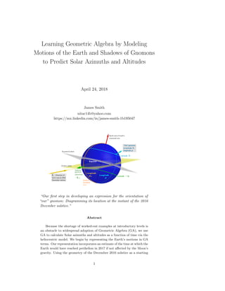
  • 1. Learning Geometric Algebra by Modeling Motions of the Earth and Shadows of Gnomons to Predict Solar Azimuths and Altitudes April 24, 2018 James Smith nitac14b@yahoo.com https://mx.linkedin.com/in/james-smith-1b195047 “Our first step in developing an expression for the orientation of “our” gnomon: Diagramming its location at the instant of the 2016 December solstice.” Abstract Because the shortage of worked-out examples at introductory levels is an obstacle to widespread adoption of Geometric Algebra (GA), we use GA to calculate Solar azimuths and altitudes as a function of time via the heliocentric model. We begin by representing the Earth’s motions in GA terms. Our representation incorporates an estimate of the time at which the Earth would have reached perihelion in 2017 if not affected by the Moon’s gravity. Using the geometry of the December 2016 solstice as a starting 1
  • 2. point, we then employ GA’s capacities for handling rotations to determine the orientation of a gnomon at any given latitude and longitude during the period between the December solstices of 2016 and 2017. Subsequently, we derive equations for two angles: that between the Sun’s rays and the gnomon’s shaft, and that between the gnomon’s shadow and the direction “north” as traced on the ground at the gnomon’s location. To validate our equations, we convert those angles to Solar azimuths and altitudes for comparison with simulations made by the program Stellarium. As further validation, we analyze our equations algebraically to predict (for example) the precise timings and locations of sunrises, sunsets, and Solar zeniths on the solstices and equinoxes. We emphasize that the accuracy of the results is only to be expected, given the high accuracy of the heliocentric model itself, and that the relevance of this work is the efficiency with which that model can be implemented via GA for teaching at the introductory level. On that point, comments and debate are encouraged and welcome. 2
  • 3. Contents 1 Introduction 8 2 Review of Relevant Information about Kepler Orbits, Earth’s orientation, and GA 10 2.1 The Gnomon and Its Uses . . . . . . . . . . . . . . . . . . . . . . 10 2.2 The Earth’s Kepler Orbit, and the Geometry of Solstices and Equinoxes . . . . . . . . . . . . . . . . . . . . . . . . . . . . . . . 13 2.2.1 The Earth’s Kepler Orbit . . . . . . . . . . . . . . . . . . 13 2.2.2 Geometry of Solstices and Equinoxes . . . . . . . . . . . . 15 2.2.3 Summary of our Review of the Earth’s Orbit and the Geometry of Equinoxes and Solstices . . . . . . . . . . . . 15 2.3 Review of GA . . . . . . . . . . . . . . . . . . . . . . . . . . . . . 17 2.3.1 Some General Comments on GA . . . . . . . . . . . . . . 18 2.3.2 Rotations and their Representations in GA . . . . . . . . 19 2.3.3 Angles Between Projected Vectors . . . . . . . . . . . . . 22 2.4 Observations on the Background . . . . . . . . . . . . . . . . . . 25 3 Detailed Formulation of Model in GA Terms 26 3.1 A Still-Unresolved Detail: How to Express ˆgL (t): The Orientation of Our Gnomon as a Function of Time . . . . . . . . . . . . . . . 26 3.1.1 Finding an Idea . . . . . . . . . . . . . . . . . . . . . . . . 27 3.1.2 Expressing the Necessary Rotations via GA . . . . . . . . 28 3.1.3 Formulating the Bivectors Needed for the Rotations . . . 30 3.1.4 Celestial North: ˆnc . . . . . . . . . . . . . . . . . . . . . . 32 3.2 Our Model, in Words and in GA Terms . . . . . . . . . . . . . . 32 4 Derivations of Formulas 34 4.1 ˆr (t), ˆrs . . . . . . . . . . . . . . . . . . . . . . . . . . . . . . . . 35 4.2 ˆMs . . . . . . . . . . . . . . . . . . . . . . . . . . . . . . . . . . . 35
  • 4. 4.3 ˆnc . . . . . . . . . . . . . . . . . . . . . . . . . . . . . . . . . . . 36 4.4 ˆgsλ . . . . . . . . . . . . . . . . . . . . . . . . . . . . . . . . . . . 36 4.5 ˆQ . . . . . . . . . . . . . . . . . . . . . . . . . . . . . . . . . . . 37 4.6 Our Gnomon’s Direction . . . . . . . . . . . . . . . . . . . . . . . 37 4.7 The Angle α (t) . . . . . . . . . . . . . . . . . . . . . . . . . . . . 37 4.8 The Angle β (t) . . . . . . . . . . . . . . . . . . . . . . . . . . . . 38 4.8.1 Denominator of the sine and cosine of β (t) . . . . . . . . 38 4.8.2 Numerators of sin β (t) and cos β (t) . . . . . . . . . . . . 38 5 Validation of the Model and Calculations 39 5.0.1 Data for Earth’s Orbit, the December 2016 Solstice, Port Moresby, and San Crist´obal de Las Casas . . . . . . . . . 39 5.1 Predictions, from Mathematical Analyses of Formulas, about Solar Zeniths and the Sun’s Azimuths at Sunrise and Sunset . . 42 5.1.1 On the March Equinox: Sunrise, Sunset, and the Move- ment of the Shadow’s Endpoint . . . . . . . . . . . . . . . 42 5.1.2 Azimuths of Sunrise and Sunset on the Solstices . . . . . 45 5.1.3 Solar Zeniths on the Solstices and Equinoxes . . . . . . . 47 5.2 Numerical Predictions of Sun’s Azimuth and Elevation as Seen from Specific Locations at Specific Times . . . . . . . . . . . . . 49 5.3 Discussion of Results from the Validations . . . . . . . . . . . . . 50 6 Conclusions 50 List of Figures 1 Students using a gnomon at a school in India ([1]). . . . . . . . 9 2 Schematic diagram of the Sun, the gnomon, and the gnomon’s shadow on the flat, horizontal surface surrounding the gnomon. . 11 3 Showing the angle α between the Sun’s rays and the shaft of the gnomon. The angle of the Sun’s altitude (also called the angle of elevation) is the complement of α. . . . . . . . . . . . . . . . . . 11 4
  • 5. 4 β is the angle of rotation from “Local North” (i.e., the direction “geographic north” as traced on the ground at the observer’s location) and the gnomon’s shadow. Later in this document, we will define the counterclockwise sense of β as positive. . . . . . . 12 5 Relationship between β and the Sun’s azimuth. . . . . . . . . . . 12 6 Schematic of the Earth’s Kepler orbit, defining the elements φ, θ, , and ˆr used in this analysis. The plane of the Earth’s orbit is known as the ecliptic. (Reproduced from [7].) . . . . . . . . . . . 14 7 The position of the 2017 perihelion with respect to the December 2016 solstice. Red arrows show the direction in which the north end of the Earth’s rotational axis points. The line connecting the positions of the Earth at the equinoxes is not perfectly perpendic- ular to the line connecting the positions at the solstices because the Earth’s axis precesses by about 1/70 ◦ per year. (Reproduced from [7].) . . . . . . . . . . . . . . . . . . . . . . . . . . . . . . . 14 8 The relationship between the Sun, Earth, ecliptic, and the Earth’s rotational axis. For our purposes, the orientation of the rotational axis is constant during a given year, and the line connecting the positions of the Earth at the equinoxes can be taken as perfectly perpendicular to the line connecting the positions at the solstices. (Reproduced from [7].) . . . . . . . . . . . . . . . . . . . . . . . . 15 9 Geometry of the equinoxes: the Earth’s axis of rotation lies within the plane that is perpendicular to the ecliptic and to the line connecting the centers of the Earth and Sun. (Reproduced from [7].) . . . . . . . . . . . . . . . . . . . . . . . . . . . . . . . . . . 16 10 Geometry of the solstices: the Earth’s axis of rotation lies within the plane that is perpendicular to the ecliptic, and which also contains the line that connects the centers of the Earth and Sun. (Reproduced from [7].) . . . . . . . . . . . . . . . . . . . . . . . . 16 11 One of the goals of our review: finding a convenient instant at which a gnomon with a known location points in an identifiable direction. At the instant of the December 2016 solstice, a gnomon along the meridian that faces the Sun directly, and whose south latitude is equal to the angle of inclination of the Earth’s rotational axis with respect to the ecliptic plane, will point in the direction −ˆr. . . . . . . . . . . . . . . . . . . . . . . . . . . . . . . . . . . . 17 12 Rotation of the vector w through the bivector angle ˆNγ, to produce the vector w . . . . . . . . . . . . . . . . . . . . . . . . . 20 13 Rotation of bivector P by the bivector angle ˆNγ to give the bivector H. . . . . . . . . . . . . . . . . . . . . . . . . . . . . . . 22 5
  • 6. 14 Reproduced from [12]. The flat, horizontal surface surrounding the gnomon is a plane tangent to the Earth (assumed spherical) at the point at which our gnomon is embedded . . . . . . . . . . 23 15 Reproduced from [12]. Note that the plane that contains the Earth’s rotational axis and the meridian on which the gnomon is located cuts the tangent plane along the direction that we have been calling “local north”. Therefore, the direction “local north” is the perpendicular projection of the direction of the Earth’s rotational axis (labeled here as ˆnc) upon the flat, horizontal surface on which our gnomon stands. . . . . . . . . . . . . . . . . 23 16 The problem treated in GA terms by [12]: the angle between the projections of two vectors, u and v, upon a unit bivector ˆN whose dual is ˆe. . . . . . . . . . . . . . . . . . . . . . . . . . . . 24 17 Our first step in developing an expression for the orientation of “our” gnomon at any time: making a diagram of its location and that of the solstice gnomon, in terms of their respective latitudes and longitudes, at the instant of the 2016 December solstice (ts). The solstice gnomon is that which points directly at the Sun at that instant; thus, its orientation is −ˆrs. . . . . . . . . . . . . . . 27 18 The second step in developing an expression for the orientation of our gnomon at any time: moving the solstice gnomon along the solstice meridian to the latitude (λ) of our gnomon. The vector of the gnomon in that position is ˆgsλ. . . . . . . . . . . . . . . . 28 19 The third step in developing an expression for the orientation of “our” gnomon at any time: moving the ˆgsλ gnomon along latitude λ longitude (µ) of our gnomon, whose orientation at the instant of the 2016 December solstice is ˆg (ts). . . . . . . . . . . . . . . . 29 20 Schematic diagram of the Earth’s Kepler orbit, showing the vec- tors ˆa and ˆb along with the unit bivector ˆC = ˆa ∧ ˆb = ˆaˆb . The arrow next to the square representing ˆC shows ˆC’s positive sense. Because that sense is in the direction of the Earth’s orbit, ˆr (t) = ˆae ˆCθ(t) . . . . . . . . . . . . . . . . . . . . . . . . . . . . . 31 21 Definition of the vector ˆc that we will use in formulating ˆMs. The set of vectors ˆa, ˆb, ˆc forms a right-handed, orthonormal basis. 31 22 Illustrating the use of ˆc, which is ˆC’s dual. The bivector (−ˆrs)∧ˆc has the characteristics that we specified earlier for ˆMs. The arrow next to the square representing ˆMs shows ˆMs’s positive sense. . 32 23 ˆQ is the rotation of ˆC through the bivector angle ˆMη. . . . . . . 34 6
  • 7. 24 The model, in GA terms. Arrows show the positive senses of the bivectors ˆQ and ˆT. Vector ˆgL (t) rotates at constant angular velocity ˆQω. The vector ˆr (t) varies with time according to the Kepler equation ((2.1)). Vector ˆnc is the dual of ˆQ. Vector ˆgL (t) is the dual of bivector ˆT (t). Not shown is the angle α between −ˆgL (t) and ˆr (t). . . . . . . . . . . . . . . . . . . . . . . . . . . . 35 25 Relative positions of meridians of Port Moresby and San Crist´obal. 40 26 Because we measure latitudes from the equator, the latitudes λ and π − λ are in fact the same latitude. . . . . . . . . . . . . . . 43 27 For simplicity, we’ve written the vector s (t) and the angles α (t) and β (t) as s, α, and β. The length, s , of the shadow cast by a gnomon of height g is g tan α. We wish to calculate the length of s’s projection upon the direction “local north” on the days of equinoxes. . . . . . . . . . . . . . . . . . . . . . . . . . . 45 28 On the day of an equinox, the trajectory of the end of the gnomon’s shadow is a straight, east-west line at the distance g tan λ from the base of the gnomon. . . . . . . . . . . . . . . . . . . . . . . . 46 List of Tables 1 Formulas for calculating azimuths according to the algebraic signs of sin β and cos β. For example, if sin β < 0 and cos β ≥ 0, then Azimuth = 180◦ + arcsin | sin β| . . . . . . . . . . . . . . . . . . 11 2 Summary of the quantities in our model. . . . . . . . . . . . . . . 33 3 Summary of the parameters used in validating the model. ”Days” are tropical days. The quantity “∆µ is µ − µs. . . . . . . . . . . 41 4 Times and dates of solstices and equinoxes for the year 2017, and the number of tropical days between each event and the December 2016 solstice. (Adapted and corrected from [7].) . . . . . . . . . . 41 5 Comparison of Sun’s azimuths and altitudes according to atellar- ium, to Those calculated from Eqs. (4.10), (4.11), (4.12), (4.13), and (4.14), as seen from Port Moresby, Papua New Guinea on three dates in 2017. All of the calculations are implemented in [16]. 51 6 Comparison of Sun’s azimuths and altitudes according to Stellar- ium, to those calculated from Eqs. (4.10), (4.11), (4.12), (4.13), and (4.14), as seen from San Crist´obal de Las Casas, Chiapas, Mexico on three dates in 2017. All of the calculations are imple- mented in [16]. . . . . . . . . . . . . . . . . . . . . . . . . . . . . 52 7
  • 8. 7 Solar azimuths and altitudes as seen from San Crist´obal de Las Casas, according to Stellarium, at five-minute intervals around UTC 4 October 2071 22:30:00 . . . . . . . . . . . . . . . . . . . . 52 1 Introduction Geometric Algebra (GA) holds promise as a means for formulating and solving problems in many different branches of mathematics and science. This document contributes to addressing one of the obstacles to GA’s wider adoption: the shortage of instructional materials that use GA to solve non-trivial problems that are accessible to students who are in high school or the first year of university. In this document, we’ll use GA for calculations that are related to gnomons (Fig. 1) —astronomical instruments of a type that dates to antiquity. Many simple, interesting experiments that use it are described in detail on line (e.g. [2]), and can be performed by students to check predictions such as those which we will make here. We will see, too, that through use of simple geometric and trigonometric relations, inferences drawn from our gnomon equations can be transformed into predictions that we can check via free planetarium software such as Stellarium ([3]). A key goal of this document is to make clear the relationship between the skill of modeling physical systems, and the nature and capabilities of the mathematical tools that are available to the modeler. The gnomon is a good example for teaching that relationship because it shows the benefits of “seeing” a system in terms of rotations—an operation to which GA is especially suited. Toward that end, our specific goals will be 1. To use GA to predict the following for any location on Earth, at any time between the December 2016 solstice and the December 2017 solstice: (a) the angle between the Sun’s rays and the gnomon; and (b) the angle between local north and the gnomon’s shadow. 2. To validate our model by comparing our predictions to results of simple gnomon observations, and to simulations made by the planetarium program Stellarium ([3]). The same calculations may be done for other years using data available at [4]. This document begins by reviewing relevant information on Kepler orbits, the geometry of the Earth’s orientation with respect to the plane of its orbit about the Sun, and GA. Based upon that review, we’ll develop a model, then derive the necessary equations. We’ll find that they are surprisingly amenable to analyses that let us test key predictions without needing to do numerical calculations. (Although we will of course do such calculations as well.) 8
  • 9. Figure 1: Students using a gnomon at a school in India ([1]). 9
  • 10. 2 Review of Relevant Information about Kepler Orbits, Earth’s orientation, and GA “Our” gnomon. To get the most out of this review, we’ll want to keep the document’s goals in mind. Let’s state them again, but this time we’ll refer to the gnomon for which we want to calculate angles, etc. as simply “our gnomon”: 1. To use Geometric algebra to predict the following, at any time between the December 2016 solstice and the December 2017 solstice: (a) the angle between the Sun’s rays and our gnomon; and (b) the angle between local north and our gnomon’s shadow. 2. To validate our model by comparing our predictions to results of simple gnomon observations, and to simulations made by the planetarium program Stellarium ([3]). Given our goals, a reasonable thing to look for during our review is some specific moment at which we can identify both of the following: the direction of the Sun’s rays, and the direction in which our gnomon is pointing. Our goal would then be to find a way to use that information to calculate, via GA, those same directions for any other instant in time that might interest us. 2.1 The Gnomon and Its Uses A gnomon is nothing more than a vertical stick, pole, or (in some cases) structure surrounded by a flat, horizontal surface of appropriate size (Fig. 2). Over the course of a year, the trajectory followed by the end of the gnomon’s shadow changes systematically from one day to the next. Most notably, that trajectory is an almost-perfect east-west line on the days of the equinoxes ([2]). Typical experiments done with gnomons include tracing that trajectory for subsequent mathematical analysis. Younger students enjoy measuring the angle β between local north and the gnomon’s shadow, and the angle α between the gnomon and a string stretched from the tip of the gnomon to the end of the shadow (Figs. 3 and 4). Figs. 3 –5 and Table 1 show how to determine the Sun’s azimuth and altitude from the angles α and β. The shaft of the gnomon can be regarded as an extension of the line segment that runs from the center of the Earth to the gnomon’s base. Please note something that will be important in our development of a model: because the Earth’s deviation from perfect sphericity is less than 0.3% ([5]), the shaft of the gnomon can be regraded as an extension of the line segment that runs from the center of the Earth to the gnomon’s base. 10
  • 11. Figure 2: Schematic diagram of the Sun, the gnomon, and the gnomon’s shadow on the flat, horizontal surface surrounding the gnomon. Figure 3: Showing the angle α between the Sun’s rays and the shaft of the gnomon. The angle of the Sun’s altitude (also called the angle of elevation) is the complement of α. Table 1: Formulas for calculating azimuths according to the algebraic signs of sin β and cos β. For example, if sin β < 0 and cos β ≥ 0, then Azimuth = 180◦ + arcsin | sin β| . sin β < 0 sin β ≥ 0 cos β < 0 360◦ − arcsin | sin β| arcsin | sin β| cos β ≥ 0 180◦ + arcsin | sin β| 180◦ − arcsin | sin β| 11
  • 12. Figure 4: β is the angle of rotation from “Local North” (i.e., the direction “geographic north” as traced on the ground at the observer’s location) and the gnomon’s shadow. Later in this document, we will define the counterclockwise sense of β as positive. Figure 5: Geometrical bases for the formulas presented in Table 1 for determining the Sun’s azimuth from sin β and cos β. Diagram is a schematic of an aerial view of a plaza in which our gnomon is set. The Sun is in the part of the sky opposite the shadow. Angle β is positive counter-clockwise from local north, and the Sun’s azimuth is positive clockwise from local north. 12
  • 13. 2.2 The Earth’s Kepler Orbit, and the Geometry of Sol- stices and Equinoxes 2.2.1 The Earth’s Kepler Orbit Fig. 6 shows key elements that we will use later: the vector ˆr from the center of the Sun to the center of the Earth; the angles θ and φ; and the vector a, from the center of the orbit through the center of the Sun, to the position of the Earth’s center at perihelion. Hestenes ([6], pp. 204-219) used GA to arrive at the well-known Kepler equation for planetary motion: 2πt T = φ − sin φ. (2.1) where T is the planet’s orbital period, t is the time elapsed since the planet was at its perihelion, and is the orbit’s eccentricity. The angle φ is in radians. For any given time t, the corresponding angle θ (t) is determined by first solving Eq. (2.1) for φ (t), after which the corresponding value of θ is found ([6], p. 219) via the relationship tan θ 2 = 1 + 1 − 1/2 tan φ 2 , (2.2) from which θ = 2 tan−1 1 + 1 − 1/2 tan φ 2 . (2.3) Ref. [7] notes that for works like the present, we must estimate what the timing and position of the Earth’s perihelion would be if the Earth’s orbit were a perfect Keplerian ellipse that is unperturbed by the gravity of other bodies, especially the Moon. Using a best-fit method, [7] estimated that the perihelion of 2017 occurred 12.93 days after the instant of the December 2016 solstice, and that that solstice therefore occurred at angle θ of 0.2301 rad before perihelion (Fig. 7). Note that Fig. 7 shows the line connecting the positions of the Earth at the equinoxes as being perpendicular the line connecting the positions at the solstices. Actually, there is a very slight non-perpendicularity because the Earth’s axis precesses by about 1/70 ◦ per year. That precession also causes a twenty-minute difference between the lengths of the Tropical year (the time between successive December solstices) and the Sidereal year (the time needed for the Earth to complete one revolution of its orbit, as measured against a fixed frame of reference such as the stars). The effects of precession will require us to be careful to use the Tropical year of 365.242 days in our calculations instead of the Sidereal year of 365.256 days, but will otherwise be negligible for our purposes. Differences between various types of year are discussed further in [8] and [9]. 13
  • 14. Figure 6: Schematic of the Earth’s Kepler orbit, defining the elements φ, θ, , and ˆr used in this analysis. The plane of the Earth’s orbit is known as the ecliptic. (Reproduced from [7].) Figure 7: The position of the 2017 perihelion with respect to the December 2016 solstice. Red arrows show the direction in which the north end of the Earth’s rotational axis points. The line connecting the positions of the Earth at the equinoxes is not perfectly perpendicular to the line connecting the positions at the solstices because the Earth’s axis precesses by about 1/70 ◦ per year. (Reproduced from [7].) 14
  • 15. Figure 8: The relationship between the Sun, Earth, ecliptic, and the Earth’s rotational axis. For our purposes, the orientation of the rotational axis is constant during a given year, and the line connecting the positions of the Earth at the equinoxes can be taken as perfectly perpendicular to the line connecting the positions at the solstices. (Reproduced from [7].) 2.2.2 Geometry of Solstices and Equinoxes During a given year, we can treat the orientation of the Earth’s equatorial plane as invariant. As shown in Fig. 8, the Earth’s rotational axis is inclined with respect to the plane of the Earth’s orbit, or ecliptic. For our purposes the orientation of the rotational axis is constant during a given year (Section 2.2.1). Therefore, we can treat the orientation of the Earth’s equatorial plane as invariant. In the common language, the terms “equinox and “solstice” refer to days, but astronomers also use those terms to refer to precise instants as well. At the instant of an equinox, the Earth’s axis of rotation lies within the plane that is perpendicular to the ecliptic and to the line connecting the centers of the Earth and Sun (Fig. 9). In contrast, at the instant of a solstice the axis lies within the plane that is perpendicular to the ecliptic, and which also contains the line that connects the centers of the Earth and Sun (Fig. 10). Using ideas similar to those given in [10], we can identify the meridian of longitude that faces the Sun directly at any given instant. The specific instant that interests us is that of the December 2016 solstice. 2.2.3 Summary of our Review of the Earth’s Orbit and the Geome- try of Equinoxes and Solstices Before we began to review this material, we had decided that as we went through each topic, we would look for some specific instant at which we could identify both of the following: (a) the direction of the Sun’s rays, and (b) the direction in which our gnomon would be pointing. 15
  • 16. Figure 9: Geometry of the equinoxes: the Earth’s axis of rotation lies within the plane that is perpendicular to the ecliptic and to the line connecting the centers of the Earth and Sun. (Reproduced from [7].) Figure 10: Geometry of the solstices: the Earth’s axis of rotation lies within the plane that is perpendicular to the ecliptic, and which also contains the line that connects the centers of the Earth and Sun. (Reproduced from [7].) 16
  • 17. Figure 11: One of the goals of our review: finding a convenient instant at which a gnomon with a known location points in an identifiable direction. At the instant of the December 2016 solstice, a gnomon along the meridian that faces the Sun directly, and whose south latitude is equal to the angle of inclination of the Earth’s rotational axis with respect to the ecliptic plane, will point in the direction −ˆr. The 2016 December solstice would seem to be a good choice. Although we don’t know the orientation of our own gnomon at that instant, we can identify the location of a gnomon that points directly at the Sun at that instant: its latitude is equal to that of the Earth’s inclination with respect to the ecliptic (Fig. 11), and its longitude is that of the meridian that faces the Sun directly. From that information, and the latitude and longitude of our own location, we should be able to determine the orientation of our gnomon at the instant of the 2016 December solstice. For our purposes, the Sun’s rays that reach the Earth are parallel to ˆr. We should also note that for our purposes, the Sun’s rays that reach the Earth are parallel to ˆr. 2.3 Review of GA At the end of the previous section (2.2.3), we identified a combination of specific gnomon location and instant in time with respect to which we should be able to express the orientation of our own gnomon at any other instant t that might interest us. Of course, we will also be able to calculate the vector ˆr for any instant t via Eqs. (2.1) and (2.3). Now, we’ll review what we’ve learned about GA so that we may learn how do the above via rotations, if practical. 17
  • 18. 2.3.1 Some General Comments on GA As both a math tutor and a self-taught student, I am all too aware of the confusion that students experience when trying to form an accurate mental model of that which a classroom teacher or the author of a textbook is striving to communicate through a combination of words, symbols, and diagrams. I hope that the following observations might help, although they are not intended to be either rigorous or complete. A sometimes-helpful recognition is that GA, as it applies to problems like the gnomon, is an attempt to capture geometric aspects of 3-D reality. The mathematicians who developed GA found that they could express that reality through concepts—of their own invention—which came to be known as vectors, bivectors, and trivectors, and through carefully-defined mathematical operations that are termed “products” of various sorts. Of course this characterization of GA is vague, but the important points are that GA is a human invention, and that the choices of which concepts and operations were to be used in the attempt to formulate and solve geometrical problems was made by human beings. Those same human beings defined the properties of the concepts; for example, they decided that any two vectors of identical length, direction, and orientation are equal, regardless of where they are located in space. (Or perhaps to be more correct, “regardless of where their endpoints are located in space”.) The originators of the concept of vectors did not include “position” among the characteristics of vectors for a very simple reason: there was no need to do so, and they saw no benefit in doing so. Similar comments apply to bivectors: their only characteristics are magni- tude (“area”, in 3-D geometry), orientation, and sense (algebraic sign). Devel- opers of GA were able to accomplish their goals without including shape and location among bivectors’ characteristics. To accomplish our own, gnomon-related goals via GA, we need to express the ecliptic plane in terms of a specific GA bivector (one to which the plane is parallel). We also need to express the relation between that bivector and the one that is used for the equatorial plane, and we need to express each of these bivectors in terms of the basis bivectors of whatever reference system we might find convenient. Rather than go into those important skills in detail here, we’ll see how to put them into practice when we develop our gnomon model, and when we derive formulas for calculating the angles α and β. Additional examples can be found in [11] and [12]. One final note before we review the relevant GA information: in this document, there are times when we will use the symbol for a given bivector (e.g., Q) to represent both the bivector itself (which is a GA object) and the plane to which that bivector is parallel. Where the meaning of the symbol is not made clear by context, we’ll state, explicitly, which meaning is intended. 18
  • 19. In somewhat the same vein, we should mention that we may talk about rotating a physical plane (such as the plane that contains the meridian of longitude on which a gnomon stands) in terms of rotating the bivector that represents it. Said meridian rotates with the Earth, so in that sense the meridian does rotate. However, when we are using the term “plane” in its strict Euclidean sense, a plane is a distinct set of points. Thus, the rotation of a plane produces a different plane, not the same plane in a different orientation. Similar comments apply to bivectors. Thus. as a the meridian rotates with the Earth, it goes into and out of alignment with a succession of bivectors. To put that differently, let’s use the symbol ˆM to denote the bivector that’s parallel to the plane that contains a certain meridian. We see immediately that the bivector that’s aligned with the plane at time t1 may be different from that with which the meridian plane is aligned at some other time t2. Therefore, “the” bivector with which the meridian is aligned is a function of time. We’ll write that function as ˆM (t). Having done so, we recognize that although ˆM (t) is a set of bivectors, each ˆM (τ) for any specific value τ of the time t is a specific, individual bivector. 2.3.2 Rotations and their Representations in GA Let’s recall that our purpose in this document is not only to calculate the angles α and β, etc., but also to learn how to employ GA effectively for the formulation and solution of certain types of problems. We expect, reasonably, that the gnomon problem will be a good one for learning how to use GA for expressing rotations, and also for determining angles between vectors. Refs. [11] and [12] treat those topics in detail, but we will present only the most-relevant and -important observations here. Rotation of a vector by a bivector angle When describing an angle of rotation in GA, we are often well advised—for sake of clarity—to write it as the product of the angle’s scalar measure (in radians) and the bivector of the plane of rotation. Following that practice, we would say that the rotation of a vector w through the angle γ (measured in radians) with respect to a plane that is parallel to the unit bivector ˆQ, is the rotation of w through the bivector angle ˆNγ. (For example, see Fig. 12.) References [6] (pp. 280-286) and [13] (pp. 89-91) derive and explain the following formula for finding the new vector, w , that results from that rotation : w = e− ˆNγ/2 [w] e ˆNγ/2 Notation: R ˆNγ (w) . (2.4) Notation: R ˆNγ (w) is the rotation of the vector w by the bivector angle ˆNγ. For our convenience later in this document, we will follow Reference [13] (p. 89) in saying that the factor e− ˆNγ/2 represents the rotation R ˆNγ. That factor 19
  • 20. Figure 12: Rotation of the vector w through the bivector angle ˆNγ, to produce the vector w . is a quaternion, but in GA terms it is a multivector. We can see that from the following identity, which holds for any unit bivector ˆB and any angle ξ (measured in radians): exp ˆBξ ≡ cos ξ + ˆB sin ξ. The representation of a rotation. Thus, e− ˆNγ/2 = cos γ 2 − ˆN sin γ 2 . (2.5) In our choice of symbols for basis vectors and bivectors, we´re following [13], p. 82. In this document, we’ll restrict our treatment of rotations to three-dimensional Geometric Algebra (G3 ). In that algebra, and using a right-handed reference system with orthonormal basis vectors ˆa, ˆb, and ˆc, we may express the unit bivector ˆN as a linear combination of the basis bivectors ˆaˆb, ˆbˆc, and ˆaˆc : ˆN = ˆaˆbnab + ˆbˆcnbc + ˆaˆcnac, in which nab, nbc, and nac are scalars, and n2 ab + n2 bc + n2 ac = 1. If we now write w as w = ˆawa + ˆbwb + ˆcwc, Eq. (2.4) becomes w = cos γ 2 − ˆN sin γ 2 [w] cos γ 2 + ˆN sin γ 2 = cos γ 2 − ˆaˆbqc + ˆbˆcqa − ˆaˆcqb sin γ 2 ˆawa + ˆbwb + ˆcwc cos γ 2 + ˆaˆbqc + ˆbˆcqa − ˆaˆcqb sin γ 2 . (2.6) Expanding the right-hand side of that result, we’d obtain 48 (!) terms, some of which would simplify to scalar multiples of ˆa, ˆb, and ˆc, and others of which will simplify to scalar multiples of the trivector ˆaˆbˆc. The latter terms would cancel, leaving an expression for w in terms of ˆa, ˆb, and ˆc . Now, we define four scalar variables: 20
  • 21. • fo = cos γ 2 ; • fab = nab sin γ 2 ; • fbc = nbc sin γ 2 ; and • fac = nac sin γ 2 . Using these variables, Eq. (2.6) becomes w = fo − ˆaˆbfab + ˆbˆcfbc + ˆaˆcfac ˆawa + ˆbwb + ˆcwc fo + ˆaˆbfab + ˆbˆcfbc + ˆaˆcfac . After expanding and simplifying the right-hand side, we obtain w = ˆa wa f2 o − f2 ab + f2 bc − f2 ac + wb (-2fofab − 2fbcfac) + wc (-2fofac + 2fabfbc) + ˆb wa (2fofab − 2fbcfac) + wb f2 o − f2 ab − f2 bc + f2 ac + wc (-2fofbc − 2fabfac) + ˆc wa (2fofac + 2fabfbc) + wb (2fofbc − 2fabfac) + wc f2 o + f2 ab − f2 bc − f2 ac . (2.7) Note that in terms of our four scalar variables fo, fab, fbc, and fac, the representation e− ˆNγ/2 of the rotation is e− ˆNγ/2 = fo − ˆaˆbfab + ˆbˆcfbc + ˆaˆcfac . (2.8) Because of the convenience with which Eq. (2.7) can be implemented, the remainder of this document will express the representations of various rotations of interest in the form of Eq. (2.8). Rotation of a bivector Fig. 13 illustrates the rotation of a bivector P by the bivector angle ˆNγ to give a new bivector, H. In his Theorem 7.5, Macdonald ([13], p. 125) states that if a blade P is rotated by the bivector angle ˆNγ, the result will be the blade R ˆNγ (P) = e− ˆNγ/2 [P] e ˆNγ/2 . (2.9) To express the result as a linear combination of the unit bivectors ˆaˆb, ˆbˆc, and ˆaˆc, we begin by writing the unit bivector ˆN as ˆN = ˆaˆbnab + ˆbˆcnbc + ˆaˆcnac, so that we may write the representation of the rotation in exactly the same way as we did for the rotation of a vector: e− ˆNγ/2 = fo − ˆaˆbfab + ˆbˆcfbc + ˆaˆcfac , with fo = cos γ 2 ; fab = nab sin γ 2 ; fbc = nbc sin γ 2 ; fac = nac sin γ 2 . Next, we write P as P = ˆaˆbpab + ˆbˆcpbc + ˆaˆcpac. Making these substitutions in Eq. (2.9), then expanding and simplifying, we obtain 21
  • 22. Figure 13: Rotation of bivector P by the bivector angle ˆNγ to give the bivector H. R ˆNγ (P) = ˆaˆb pab 1 − 2f2 bc − 2f2 ac +2 [fab (fbcpbc + facpac) + fo (facpbc − fbcpac)]} + ˆbˆc pbc 1 − 2f2 ab − 2f2 ac +2 [fbc (fabpab + facpac) + fo (fabpac − facpab)]} + ˆaˆc pac 1 − 2f2 ab − 2f2 bc +2 [fac (fabpab + fbcpbc) + fo (fbcpab − fabpbc)]} . (2.10) 2.3.3 Angles Between Projected Vectors Ref. [12] treats this topics in detail, noting that the direction that we have been calling “local north” is the perpendicular projection of the Earth’s rotational axis upon a plane that is tangent to the Earth’s surface (assumed perfectly spherical) at the gnomon’s location (Figs. 14 and 15). Another observation in [12] is that the gnomon’s shadow is the the projection of ˆr upon that same plane. Thus, our angle β is the angle between those two projections. Ref. [12] considered precisely that sort of problem in GA terms: the angle between the projections of two vectors, u and v, upon a unit bivector ˆP whose dual is ˆe (Fig. 16). Writing these elements as • u = ˆaua + ˆbub + ˆcuc, 22
  • 23. Figure 14: Reproduced from [12]. The flat, horizontal surface surrounding the gnomon is a plane tangent to the Earth (assumed spherical) at the point at which our gnomon is embedded . Figure 15: Reproduced from [12]. Note that the plane that contains the Earth’s rotational axis and the meridian on which the gnomon is located cuts the tangent plane along the direction that we have been calling “local north”. Therefore, the direction “local north” is the perpendicular projection of the direction of the Earth’s rotational axis (labeled here as ˆnc) upon the flat, horizontal surface on which our gnomon stands. 23
  • 24. Figure 16: The problem treated in GA terms by [12]: the angle between the projections of two vectors, u and v, upon a unit bivector ˆN whose dual is ˆe. • v = ˆava + ˆbvb + ˆcvc, • e = ˆaea + ˆbeb + ˆcec, and • ˆN = ˆaˆbnab + ˆbˆcnbc + ˆaˆcnac = ˆaˆbec + ˆbˆcea − ˆaˆceb , [12] found that sin γ = (uavb − ubva) nab + (ubvc − ucvb) nbc + (uavc − ucva) nac u · ˆN v · ˆN , = (uavb − ubva) ec + (ubvc − ucvb) ea − (uavc − ucva) eb u · ˆN v · ˆN , (2.11) where u · ˆN and v · ˆN are the square roots of the expressions u · ˆN 2 = u2 a 1 − e2 a + u2 b 1 − e2 b + u2 c 1 − e2 c − 2uaubeaeb − 2ubucebec − 2uauceaec , (2.12a) and v · ˆN 2 = v2 a 1 − e2 a + v2 b 1 − e2 b + v2 c 1 − e2 c − 2vavbeaeb − 2vbvcebec − 2vavceaec . (2.12b) 24
  • 25. Those expressions reduce to u · ˆN 2 = u2 − (u · ˆe) 2 = u2 a + u2 b + u2 c − (uaea + ubeb + ucec) 2 , (2.13a) and v · ˆN 2 = v2 − (v · ˆe) 2 = v2 a + v2 b + v2 c − (vaea + vbeb + vcec) 2 . (2.13b) Ref. [12] also found that cos γ = u · ˆN v · ˆN 0 u · ˆN v · ˆN , (2.14) where u · ˆN v · ˆN 0 = uava 1 − n2 bc + ubvb 1 − n2 ac + ucvc 1 − n2 ab − (uavc + ucva) nabnbc + (ubvc + ucvb) nabnac + (uavb + ubva) nbcnac, = uava 1 − e2 a + ubvb 1 − e2 b + ucvc 1 − e2 c − (uavc + ucva) eaec − (ubvc + ucvb) ebec − (uavb + ubva) eaeb. (2.15) For our gnomon problem, the relevance of the above equations is that (1) the unit vector that points from the center of the Earth to the tip of the gnomon is also the dual of the bivector that is parallel to the plane on which the gnomon is erected, and (2) the direction of the Sun’s rays is ˆr (Section 2.2.3). 2.4 Observations on the Background Below, we’ll add the subscript L to ˆg to denote the orientation of “our” gnomon, and have used ˆgL (t) instead of simply ˆgL in recognition of the fact that the orientation of the gnomon on a rotating Earth is a function of time. One purpose of our review was to find a specific instant at which we could identify both of the following: the direction of the Sun’s rays, and the direction in which our gnomon is pointing. Fig. 11, showing the geometry of the 2016 December solstice, seems to provide a good starting point. We can now attempt to use that information to calculate, via GA, the direction of the Sun’s rays and our own gnomon at any other instant. To express the following additional observations more conveniently, we’ll denote the unit vector of the direction from the Earth’s center to the tip of our 25
  • 26. gnomon as ˆgL (t), where t is the time elapsed since the Earth was at perihelion. We’ll also note that ˆr, too, is a function of t, and write it as ˆr (t) . Similarly, α is α (t), and β is β (t). Here, then, are the observations that might be most useful: 1. The key elements in our problem appear to be the direction of the Sun’s rays; the ecliptic plane; the Earth’s axis of rotation; and the Earth’s equatorial plane. 2. The ecliptic plane, equatorial plane, and direction of the Earth’s rotational axis can all be taken as invariant. 3. So that we may use the Kepler equation and its various transformations, we are well advised to define the time t as Kepler did. That is, t = 0 when the Earth is at perihelion. 4. The direction of the Sun’s rays can be taken as ˆr (t). 5. From Figs. 3 and 11, we can deduce that cos α (t) = ˆr (t) · [−ˆgL (t)]. 6. The direction “Local north” is the projection of the Earth’s rotational axis upon the plane that is tangent to the Earth at the point at which our gnomon is fixed. Because of the Earth’s rotation, local north is a function of t. 7. The gnomon’s shadow is the projection of ˆr (t) upon that same plane. 8. To find the angle β (t), given ˆr (t) and ˆgL (t), we can use Eqs. (2.11) and (2.14). 9. To find ˆr (t) at any given time, we can use Eqs. (2.1) and (2.2) . Hence, we now have all we need for deriving formulas expressing angles α and β for our gnomon at any time, if we can express the orientation of the gnomon itself as a function of time. 3 Detailed Formulation of Model in GA Terms 3.1 A Still-Unresolved Detail: How to Express ˆgL (t): The Orientation of Our Gnomon as a Function of Time One of the purposes of this document is to show one way in which we might puzzle through a problem like the gnomon, to arrive at a workable model and solution strategy. Therefore, rather than just present a formula for ˆgL (t), we’ll struggle with the problem a bit. 26
  • 27. Figure 17: Our first step in developing an expression for the orientation of “our” gnomon at any time: making a diagram of its location and that of the solstice gnomon, in terms of their respective latitudes and longitudes, at the instant of the 2016 December solstice (ts). The solstice gnomon is that which points directly at the Sun at that instant; thus, its orientation is −ˆrs. 3.1.1 Finding an Idea At this moment, our question is, “What do we want?” The answer is, “An expression for ˆgL (t).” So: what things did we note during our review, that might be useful? Here are three possibilities: • Via GA, we can formulate, readily, rotations about a given axis or by a given bivector angle. • The Earth rotates about its axis at a constant scalar angular velocity ω. • We identified Fig. 11 as a promising starting-point for our present task. An additional consideration might be that we should express the location of “our” gnomon via its latitude λ and its longitude µ. Thinking through the above observations. we might draft something like Fig. 17, and conceive the follow overall plan: 1. First, we’ll derive an expression for the orientation of “our” gnomon at the instant of the 2016 December solstice. We’ll denote that instant by ts. Thus, the vector that gives the orientation of our gnomon at that instant is ˆg (ts). 2. To find an expression for the orientation of our gnomon at any other time t, we’ll rotate ˆg (ts) about the Earth’s axis via GA. 27
  • 28. Figure 18: The second step in developing an expression for the orientation of our gnomon at any time: moving the solstice gnomon along the solstice meridian to the latitude (λ) of our gnomon. The vector of the gnomon in that position is ˆgsλ. We should make a note to ourselves here, reminding us that we’ll want to follow the usual convention of expressing northern latitudes as positive angles, and southern latitudes as negative ones. Now, let’s flesh out that plan a bit. At this stage, we may alternate between thinking in terms of “moving gnomons around on the globe” in Fig. 17, and rotating the corresponding vectors. So: how can we identify ˆg (ts)? One way is to recognize that we could do so by moving the solstice gnomon along meridians of longitude and parallels of longitude to the position of our gnomon. Thus, we would first slide the solstice gnomon along the solstice meridian, to the latitude (λ) of our gnomon (Fig. 18). In GA terms, that movement is the rotation of the vector −ˆrs through the scalar angle λ − (−η) , = λ + η. We’ll call the resulting vector ˆgsλ, and identify the bivector for that rotation later. Another note to ourselves: we’ll follow the usual convention of expressing eastern longitudes as positive angles, and western longitudes as negative ones. Having “moved the solstice gnomon to our latitude”, and called the result ˆgsλ, we’ll now slide ˆgsλ along our latitude until it stands on our meridian of longitude, µ (Fig. 19). In GA terms, that movement is a rotation by the scalar angle µ − µs about the Earth’s axis. The result will be the vector that we called ˆg (ts): the orientation of our gnomon at the instant of the 2016 December solstice. Now, to find the orientation of our gnomon at any other instant, t, we just rotate ˆg (ts) about the Earth’s axis by the angle ω (t − ts). 3.1.2 Expressing the Necessary Rotations via GA How might we formulate in GA terms the rotations that we described in the previous section? For the “sliding” along the solstice meridian, a reasonable idea is to define a unit bivector ˆMs that’s parallel to the plane containing that meridian, and whose positive sense is that of the rotation from −ˆrs to 28
  • 29. Figure 19: The third step in developing an expression for the orientation of “our” gnomon at any time: moving the ˆgsλ gnomon along latitude λ longitude (µ) of our gnomon, whose orientation at the instant of the 2016 December solstice is ˆg (ts). ˆnc. Having defined ˆMs in this way, ˆgsλ is the rotation of −ˆrs through the bivector angle ˆMs (λ + η). (That is, through the scalar multiple λ + η of the unit bivector ˆMs.) The representation of that rotation ([13], p. 89) would then be Z1 = e− ˆMs (λ + η) /2. For the rotations about the Earth’s axis, we’ll define a unit vector ˆQ that’s parallel to the equator. What should we choose as ˆQ’s positive sense? The direction of the Earth’s rotation about its axis is a good choice, all the more so because the dual of a ˆQ that’s so defined is none other than the vector ˆnc. Using this definition of ˆQ, the representation of the rotation of ˆgsλ from the solstice meridian to our own meridian to the longitude of our meridian at time ts is Z2 = e− ˆQ (µ − µs) /2. The subsequent rotation of our meridian (and thus of our gnomon) from the time ts to any other time t is represented by Z3 = e− ˆQω (t − ts) /2. Putting the preceding ideas together, we see that ˆgL (t) is the result of the rotation of −ˆrs by the composite of the three above-described rotations. As explained in [13], p. 125, the representation of that composite rotation is the product Z3Z2Z1 of their respective rotations: Z3Z2Z1 = e− ˆQω (t − ts) /2 e− ˆQ (µ − µs) /2 e− ˆMs (λ + η) /2 = e− ˆQ [µ − µs + ω (t − ts)] /2 e− ˆMs (λ + η) /2 . To make that result more convenient, we’ll define k (µ, t) = µ − µs + ω (t − ts), giving Z3Z2Z1 = e− ˆQk (µ, t) /2 e− ˆMs (λ + η) /2 Because that result is the representation of the rotation that produces ˆgL (t) 29
  • 30. from −ˆrs, ˆgL (t) = e− ˆQk (µ, t) /2 e− ˆMs (λ + η) /2 [−ˆrs] e ˆMs (λ + η) /2 e ˆQk (µ, t) /2 The above having been said, we’re under no obligation to calculate ˆgL (t) directly from ˆrs. Depending upon the complexity of the expressions that arise when we make substitutions for ˆrs, ˆMs, and ˆQ, we might instead choose to first derive an expression for ˆgsλ from ˆrs, ˆgsλ = e− ˆMs (λ + η) /2 [−ˆrs] e ˆMs (λ + η) /2 , (3.1) after which we would calculate ˆgL (t) via ˆgL (t) = e− ˆQk (µ, t) /2 [ˆgsλ] e ˆQk (µ, t) /2 . (3.2) Other reasons for choosing this route include the possibility of gaining greater insight into the relationships between the calculations and the physical phenom- ena, and the desire to check the results of each step to make sure that they make sense. 3.1.3 Formulating the Bivectors Needed for the Rotations In the previous section, we used GA’s capacities for formulating rotations to express ˆgL (t) in terms of the vector ˆrs (= ˆr (ts)) and the time-invariant bivectors ˆMs and ˆQ. Now, let’s develop expressions for those bivectors in terms of the vectors ˆa and ˆb of the Earth’s Kepler orbit. Our purpose in doing so is to facilitate the numerical calculations of α (t) and β (t) that we will wish to make. ˆa ∧ ˆb = ˆaˆb because ˆa ⊥ ˆb. In Fig. 20, we introduce the unit bivector ˆC = ˆa ∧ ˆb = ˆaˆb . It’s parallel to the ecliptic plane, and its positive sense is in the direction of the Earth’s orbit. Thus, for any time t, ˆr (t) = e− ˆCθ(t)/2 [ˆa] e ˆCθ(t)/2 = ˆae ˆCθ(t) , (3.3) because ˆa is parallel to ˆC. In particular, ˆrs = ˆae ˆCθs . We decided in the previous section to define ˆMs as the unit bivector that is parallel to the solstice meridian, and whose positive sense is in the direction of the rotation from −ˆrs ˆnc . Examining Figs. 21–22, we see that those characteristics are possessed by the bivector (−ˆrs) ∧ ˆc, where ˆc is ˆC’s dual. Comparing Figs. 20 and 22, we also see that the set of vectors ˆa, ˆb, ˆc forms a right-handed, orthonormal basis—quite a favorable development for our purposes. Thus, we define ˆMs = (−ˆrs) ∧ ˆc = −ˆrsˆc, (3.4) 30
  • 31. Figure 20: Schematic diagram of the Earth’s Kepler orbit, showing the vectors ˆa and ˆb along with the unit bivector ˆC = ˆa ∧ ˆb = ˆaˆb . The arrow next to the square representing ˆC shows ˆC’s positive sense. Because that sense is in the direction of the Earth’s orbit, ˆr (t) = ˆae ˆCθ(t) . Figure 21: Definition of the vector ˆc that we will use in formulating ˆMs. The set of vectors ˆa, ˆb, ˆc forms a right-handed, orthonormal basis. 31
  • 32. Figure 22: Illustrating the use of ˆc, which is ˆC’s dual. The bivector (−ˆrs) ∧ ˆc has the characteristics that we specified earlier for ˆMs. The arrow next to the square representing ˆMs shows ˆMs’s positive sense. because ˆrs ⊥ ˆc. With ˆMs defined in this way, ˆQ, which we need for rotations about the Earth’s axis, is just the rotation of ˆC through the bivector angle ˆMη Fig. 23: ˆQ = e− ˆMsη/2 ˆC e ˆMsη/2 . (3.5) 3.1.4 Celestial North: ˆnc From Fig. 23, we can see that the rotation from ˆc to ˆnc is the same as that from ˆMs to ˆQ. Therefore, having formulated ˆMs, we can now express ˆnc readily as the rotation of ˆc by the bivector angle ˆMsη: ˆnc = e− ˆMsη/2 [ˆc] e ˆMsη/2 . (3.6) We could also formulate it as dual of ˆQ. 3.2 Our Model, in Words and in GA Terms We developed our model and defined its variables in the course of “puzzling- through” the gnomon problem, so we should take time now to summarize and organize (Table 2 ) before moving on to derive equations for the angles α and β. 32
  • 33. Table 2: Summary of the quantities in our model. Symbol Description ˆa, ˆb, ˆc The right-handed, orthonormal basis of our reference system. t Time, per Kepler equation. When t = 0, Earth is at perihelion. ts Value of t at the instant of the 2016 December solstice. η The angle of the equator with respect to the ecliptic. Positive if in the positive sense of ˆMs. λ Our (that is, our gnomon’s) latitude. Positive in the Northern Hemisphere, negative in the Southern Hemisphere. µ Our longitude, with East longitudes taken as positive. µs Value of µ for the “solstice meridian”: that which faced the Sun directly at the December 2016 solstice. ω Angular velocity of the Earth’s rotation about its own axis. k (µ, t) = µ − µs + ω (t − ts). r (t) Vector from Sun’s center to Earth’s center at time t. Direction of Sun’s rays is approximated as equal to ˆr (t). ˆrs = ˆr (ts). θ (t) Angle from ˆa to ˆr (t). Positive in the direction of the Earth’s orbit, and thus if in the positive sense of ˆC. θs = θ (ts) . ˆC Unit bivector = ˆaˆb of the ecliptic plane. Assumed constant. ˆMs Unit bivector of the solstice meridian. Equal to −ˆrsˆc. ˆQ Unit bivector of Earth’s equatorial plane. Assumed constant; equal to rotation of ˆQ by ˆMsη ˆnc “Celestial North”: the direction from the center of the Earth to the Geographic North Pole. ˆnL (t) “Local north”: the direction, at t, of “north” at our location. ˆgsλ Direction, at time ts, of a gnomon at latitude λ, longitude µs. ˆgL (t) Direction, t, from base of our gnomon to its tip. This vector is ˆT (t)’s dual. ˆT (t) Unit bivector parallel to the plane that, at time t, is tangent to Earth’s surface at base of our gnomon. ˆT (t)’s dual is ˆgL (t). ˆs (t) Direction, at time t, from base of our gnomon to tip of its shadow. α (t) Angle between gnomon’s shaft and Sun’s rays at instant t. β (t) Angle of rotation from ˆnL (t) to ˆs (t). 33
  • 34. Figure 23: ˆQ is the rotation of ˆC through the bivector angle ˆMη. Our model is that the Earth is perfectly spherical, and orbits the Sun according to the Kepler model. The direction of the Sun’s rays is the same as the direction ˆr (t) from the center of the Sun to the center of the Earth. The Earth’s equatorial plane is inclined by angle η (assumed constant) with respect to the ecliptic. The Earth rotates at constant angular velocity ω. At the instant of the 2016 December solstice, the longitude that faces the Sun directly is µs. Our gnomon is located at latitude λ, longitude µ, and casts a shadow upon a plane that is tangent to the Earth at that same location. We wish to be able to calculate, for any time t, the angle between the Sun’s rays and the gnomon, and the angle between the direction “local north” and the gnomon’s shadow. In GA terms (Fig. 24), vector ˆgL (t) rotates at constant angular velocity ˆQω. The vector ˆr (t) varies with time according to the Kepler equation ((2.1)). Vector ˆnc is the dual of ˆQ. Vector ˆgL (t) is the dual of bivector ˆT (t). We wish to be able to calculate, for any time t, (1) the angle between the vectors ˆgL (t) and ˆr (t), and (2) the angle of rotation from ˆnc’s projection upon ˆT (t) to ˆr (t)’s projection upon ˆT (t). 4 Derivations of Formulas Several of the derivations use formulas that are developed in Section 2.3.2, and implemented in Maxima in [14]. 34
  • 35. Figure 24: The model, in GA terms. Arrows show the positive senses of the bivectors ˆQ and ˆT. Vector ˆgL (t) rotates at constant angular velocity ˆQω. The vector ˆr (t) varies with time according to the Kepler equation ((2.1)). Vector ˆnc is the dual of ˆQ. Vector ˆgL (t) is the dual of bivector ˆT (t). Not shown is the angle α between −ˆgL (t) and ˆr (t). 4.1 ˆr (t), ˆrs This vector is the rotation of ˆa through the bivector angle ˆCθ (t). Thus (Eq. (3.3)), ˆr (t) = ae ˆCθ(t) = ˆaeˆaˆbθ(t) = ˆa cos θ (t) + ˆaˆb sin θ (t) = ˆa cos θ (t) + ˆb sin θ (t) . (4.1) Specifically, ˆrs = ˆr (ts) = ˆa cos θs + ˆb sin θs. (4.2) 4.2 ˆMs From Eq. (3.4), ˆMs = −ˆrsˆc. Thus, using the expression for −ˆrs from Eq. (4.2), ˆMs = − ˆa cos θs + ˆb sin θs ˆc = −ˆbˆc sin θs − ˆaˆc cos θs. (4.3) 35
  • 36. ˆMs is also the rotation of the bivector ˆcˆa through the bivector angle ˆQθs: ˆMs = e −C θs 2 [ˆcˆa] e C θs 2 = cos θs 2 − ˆaˆb sin θs 2 [ˆcˆa] cos θs 2 + ˆaˆb sin θs 2 = −ˆbˆc sin θs − ˆaˆc cos θs. 4.3 ˆnc This vector is the rotation of ˆc by the bivector angle ˆMsη. We’ll calculate ˆnc using Eqs. (2.7) and (2.8). To do so, we need to write the representation of the rotation by ˆMsη in the form fo − ˆaˆbfab + ˆbˆcfbc + ˆaˆcfac : e − ˆMs η 2 = cos η 2 − −ˆbˆc sin θs − ˆaˆc cos θs sin η 2 = cos η 2 − ˆbˆc sin θs sin η 2 − ˆaˆc cos θs sin η 2 , (4.4) so fo = cos η 2 , fab = 0, fbc = − sin θs sin η 2 , and fac = − cos θs sin η 2 . Therefore, ˆnc = ˆa sin(η) cos θs + ˆb sin(η) sin θs + ˆc cos(η). (4.5) 4.4 ˆgsλ The vector ˆgsλ is the rotation of −ˆrs by the bivector angle ˆMs (η + λ). As was the case for calculating ˆnc, we need to write the representation of our rotation in the form fo − ˆaˆbfab + ˆbˆcfbc + ˆaˆcfac : e − ˆMs η + λ 2 = cos η + λ 2 − −ˆbˆc sin θs − ˆaˆc cos θs sin η + λ 2 = cos η + λ 2 − ˆbˆc sin θs sin η + λ 2 − ˆaˆc cos θs sin η + λ 2 , (4.6) so fo = cos η + λ 2 , fab = 0, fbc = − sin θs sin η + λ 2 , and fac = − cos θs sin η + λ 2 . Therefore, ˆgsλ = ˆa [− cos θs cos (η + λ)] + ˆb [− sin θs cos (η + λ)] + ˆc [sin (η + λ)] . (4.7) 36
  • 37. 4.5 ˆQ ˆQ is ˆC rotated through the bivector angle ˆMsη: ˆQ = e − ˆMs η 2 ˆC e ˆMs η 2 = cos η 2 − −ˆbˆc sin θs − ˆaˆc cos θs sin η 2 ˆaˆb cos η 2 + −ˆbˆc sin θs − ˆaˆc cos θs sin η 2 = ˆaˆb cos η + ˆbˆc cos θs sin η − ˆaˆc sin θs sin η. (4.8) 4.6 Our Gnomon’s Direction: ˆgL (t) This vector is the rotation of ˆgsλ by the bivector angle ˆQk (µ, t). The pa- rameters of our rotation are f0 = cos k (µ, t) 2 , fab = cos η sin k (µ, t) 2 , fbc = cos θs sin(η) sin k (µ, t) 2 , fac = − sin θs sin(η) sin k (µ, t) 2 . Therefore, from Eqs. (2.7) and (2.8), ˆgL (t) = ˆa {sin θs cos λ sin k (µ, t) − cos θs cos (η + λ) + cos θs cos η cos λ [1 − cos k (µ, t)]} +ˆb {sin θs cos η cos λ [1 − cos k (µ, t)] − sin θs cos (η + λ) − cos θs cos λ sin k (µ, t)} +ˆc {sin (η + λ) − sin η cos λ [1 − cos k (µ, t)]}. (4.9) 4.7 The Angle α (t) As noted in Section 2.4, α (t) is the angle of rotation from -ˆgL (t) to ˆr (t). A gnomon is a device for producing shadows, which occur only when the Sun is above the horizon; in other words, when the inner product of -ˆgL (t) · ˆr (t) is positive. Having ensured that, the only characteristic of α (t) that interests us is its magnitude. Therefore, all we need to know is α (t)’s cosine, which is equal to the inner product ˆu · ˆv. Therefore, cos α (t) = [-ˆgL (t)] · ˆr (t). We’ve developed expressions for these two vectors (Eqs. (4.9) and (4.1), we find that cos α = {cos (η + λ) − cos η cos λ [1 − cos k (µ, t)]} cos (θt − θs) + cos λ sin (θt − θs) sin k (µ, t) . (4.10) Some comments upon that equation: At the instant ts of the December solstice, θ (t) = θs. In addition, for points along the meridian that’s aligned with the Sun at that time (e.g., points along Ms), k (µ, t) = 0. Therefore, along that meridian and at that instant, Eq. (4.10) reduces to cos α (ts) = cos (η + λ). Does our answer make sense?Does that result make sense? 37
  • 38. 4.8 The Angle β (t) We will find β (t) from its sine and cosine, which we will calculate according to Section 2.3.3. 4.8.1 Denominator of the sine and cosine of β (t) This denominator is the product of ˆnc · ˆT (t) and [ˆr (t)] · ˆT (t) . We’ll treat each of those quantities in turn. The norm ˆnc · ˆT (t) . To calculate this norm, we will use Eq. (2.12), which expresses the norm of a vector’s projection upon a bivector in terms of that bivector’s dual. In our case, the dual of ˆT (t) is ˆgL (t) (Eq. (4.9)), and ˆnc is given by Eq. (4.3). The result, as given in [14], is ˆnc · ˆT (t) = |cos λ|. However, |cos λ| = cos λ in our model because −π/2 ≤ λ ≤ π/2 . Thus, ˆnc · ˆT (t) = cos λ. (4.11) Does our answer make sense? A surprisingly simple result. Does it make sense? Let’s look at Fig. 14. We can deduce that the angle between ˆnc and ˆT (t) is either λ or 180◦ + λ. Because ˆnc is a unit vector, the magnitude of RˆT (ˆnc) (i.e., of ˆnc’s projection upon ˆT (t)) is indeed cos λ. As explained in [12], ˆnc · ˆT (t) evaluates to a vector that is a 90◦ rotation of RˆT ( ˆnc), with no change in the latter’s magnitude. Therefore, ˆnc · ˆT (t) = RˆT (ˆnc) = cos λ. The norm [ˆr (t)] · ˆT (t) As shown in [14], using (4.1)’s expression for ˆr (t) in Eq. (2.12) yields a result that I was not able to reduce to a simple form. Nor was I able to do so by starting from the observation that because ˆr (t) is a unit vector, [ˆr (t)] · ˆT (t) 2 = 1 − {[ˆr (t)] · [ˆgL (t)]} 2 , Does our answer make sense? What should [ˆr (t)] · ˆT (t) be when t = ts? Note that when t = ts, θt = θs and k (µ, t) = 0. from which ( [14]) [ˆr (t)] · ˆT (t) 2 = 1 − {[cos η cos λ (1 − cos k (µ, t)) − cos (η + λ)] cos [θt − θs] − cos λ sin k (µ, t) sin [θ (t) − θs]} 2 . (4.12) 4.8.2 Numerators of sin β (t) and cos β (t) Eqs. (4.5), (4.1), and (4.9) (respectively) present the expressions that we developed for ˆnc, ˆr (t), and ˆgL (t). To calculate the numerators of sin β (t) and cos β (t), we will substitute those expressions for (respectively)u, v, and ˆe in Eqs. (2.11) and (2.14). Those equations are implemented in [14], which is the source from which we cite the results presented in the paragraphs that follow. 38
  • 39. Note that cos λ (which is ˆnc · ˆT (t) , Eq. (4.11)) is a factor of every term in both numerators. Numerator of sin β (t) As given in [12], the numerator of sin β (t) is Numerator of sin β (t) = cos λ cos k (µ, t) sin [θ (t) − θs] − cos η cos λ sin k (µ, t) cos [θ (t) − θs] . (4.13) Numerator of cos β (t) As given in [12], the numerator of sin β is Numerator of cos β (t) = cos λ sin λ sin k (µ, t) sin [θ (t) − θs] + cos η cos λ sin λ cos k (µ, t) cos [θ (t) − θs] + sin η cos2 λ cos [θ (t) − θs] . (4.14) 5 Validation of the Model and Calculations We’ll validate the model and calculations in two ways: (1) by deducing, from mathematical analyses of our equations for α (t) and β (t), the latitudes at which solar zeniths occur on the equinoxes and solstices, and the azimuths at which the Sun sets on those dates; and (2) by making numerical predictions of the Sun’s azimuth and altitude as seen at specific times from Port Moresby, Papua New Guinea, and from San Crist´obal de Las Casas, Chiapas, Mexico. Those locations were chosen because they lie on opposite sides of the equator, and also on opposite sides of the meridian that faces the Sun at the instant of the December 2016 solstice. Thus, their values of λ and µ − µs are of opposite algebraic signs (Fig. 25). For that reason, they provide a way of detecting sign errors in our calculations. Because the two cities also lie within the Tropics of their respective hemispheres, the Sun will be in the northern half of the sky during one part of the year, and in the southern half during the other. That characteristic will enable us to detect other types of errors, if present. 5.0.1 Data for Earth’s Orbit, the December 2016 Solstice, Port Moresby, and San Crist´obal de Las Casas The Earth and its orbit Reference [5] gives the orbit’s eccentricity ( ) as 0.1671022, and its orbital period, T, 365.242 tropical days. The inclination of the Earth’s rotational axis is 23.44◦ . At the December solstice, the axis is pointed away from the Sun, so the algebraic sign of that angle is positive. Thus, η = 23.44◦ . Identifying the Earth’s rotational angular velocity, ω, requires some thought. As noted in [8], the Earth rotates by slightly more than 360◦ during one tropical day. Over the course of a full year, that slight 39
  • 40. Figure 25: Relative positions of the meridians of Port Moresby and San Crist´obal de Las Casas with respect to the Greenwich Meridian and the meridian that faces the Sun directly at the instant of the December 2016 solstice. Note that ∆µ = µ − µs. daily excess adds up to one full rotation. Therefore, the Earth makes 366.242 rotations of 2π radians each in 365.242 tropical days, from which ω = 6.3004 radians/tropical day. The December 2016 solstice Reference [7] found that for the December 2016 solstice, which occurred at UTC 21 December 2016 10:44:44, θs = −0.230099 radians, and ts = −12.9379 tropical days. Using the planetarium program Stellarium ([3]), I found that the meridian of longitude that faced the Sun directly at the instant of the solstice was E 18◦ 33 (-0.32376 radians, according to the sign convention used in our model): approximately that of Stockholm, Sweden and Cape Town, Republic of South Africa. Port Moresby and San Crist´obal de Las Casas According to [3], Port Moresby’s latitude and longitude are S9◦ 26 35.30 E147◦ 10 46.98 , while San Crist´obal’s are N16◦ 44 12.00 W92◦ 38 18.01 . Therefore, Port Moresby’s value of µ − µs is +128◦ 37 , or 2.2450 radians, and San Crist´obal´s is -1.9406 radians. Summary of the parameters used in validating the model Tables 3 and 4 summarize the relevant data. 40
  • 41. Table 3: Summary of the parameters used in validating the model. ”Days” are tropical days. The quantity “∆µ is µ − µs. Parameters of the Earth and its orbit T, days η, radians ω, radians/day 0.16710 365.242 0.40911 6.30039 Parameters of the December 2016 solstice Date (UTC) θs, radians ts, days µs, radians 21/12/2016 10:44:00 -0.23010 -12.938 0.32376 Parameters of Port Moresby and San Crist´obal de Las Casas λ, radians ∆µ, radians Port Moresby -0.16481 2.2450 San Crist´obal 0.29211 -1.9406 Table 4: Times and dates of solstices and equinoxes for the year 2017, and the number of tropical days between each event and the December 2016 solstice. (Adapted and corrected from [7].) Event UTC Time and date ([4]) t − ts, days Dec. 2016 solst 21/12/2016 10:44:00 0.000 Mar. 2017 equin 20/03/2017 10:29:00 88.987 June 2017 solst 21/06/2017 04:24:00 181.736 Sept. 2017 equin 22/09/2017 20:02:00 275.388 Dec. 2017 solst 21/12/2017 16:28:00 365.239 41
  • 42. 5.1 Predictions, from Mathematical Analyses of Formu- las, about Solar Zeniths and the Sun’s Azimuths at Sunrise and Sunset For convenience, we’ll repeat Eqs. (4.10), (4.13), and (4.14) here: cos α (t) = {cos (η + λ) − cos η cos λ [1 − cos k (µ, t)]} cos (θt − θs) + cos λ sin (θt − θs) sin k (µ, t) (5.1) Numerator of sin β (t) = cos λ cos k (µ, t) sin [θ (t) − θs] − cos η cos λ sin k (µ, t) cos [θ (t) − θs] . (5.2) Numerator of cos β (t) = cos λ sin λ sin k (µ, t) sin [θ (t) − θs] + cos η cos λ sin λ cos k (µ, t) cos [θ (t) − θs] + sin η cos2 λ cos [θ (t) − θs] . (5.3) We’ll also recall that from Eqs. (4.11) and (4.12), the denominator of sin β and cos β is the product of cos λ and the square root of 1 − {[cos η cos λ (1 − cos k (µ, t)) − cos (η + λ)] cos [θt − θs] − cos λ sin k (µ, t) sin [θ (t) − θs]} 2 . (5.4) Now, we’ll analyze those formulas to find out what they predict for the azimuths and latitudes of sunrises, sunsets, and solar zeniths. In some cases, we’ll also find it useful to recognize that because we measure latitudes from the equator, the latitudes λ and π − λ are in fact the same latitude (Fig. 26). 5.1.1 On the March Equinox: Sunrise, Sunset, and the Movement of the Shadow’s Endpoint The two key ideas in these analyses are that the Sun’s rays are parallel to the Earth’s surface at sunrise and sunset (thereforecos α = 0), and that at the instant of the March equinox, θ (t) − θs = π/2. Combining those two observations, we can deduce from Eq. (5.1) that at the instant of the March equinox sunrise, cos λ sin k (µ, t) = 0. Thus, we have only two possibilities: either cos λ = 0, or sin k (µ, t) = 0. The condition cos λ = 0 would mean that at the instant of an equinox, sunset is occurring only at the north and south poles. We reject that possibility, because we know that sunsets are never experienced at only one single, precise latitude. Thus, we conclude that sin k (µ, t) = 0, and cos k (µ, t) = ±1. 42
  • 43. Figure 26: Because we measure latitudes from the equator, the latitudes λ and π − λ are in fact the same latitude. The azimuth at which the Sun rises and sets on the equinoxes Sub- stituting sin k (µ, t) = 0 and θ (t) − θs = π/2 in Eq. (5.4), we find that the denominator of sin β is cos λ. Next, substituting sin k (µ, t) = 0, θ (t)−θs = π/2, and cos k (µ, t) = ±1 in Eq. (5.2), the numerator of sin β is ± cos λ. Thus, sin β = ±1. What is the physical interpretation of that result? Let’s go back and re-examine the condition sin k (µ, t) = 0. That condition is met by either of k (µ, t) = 0 or k (µ, t) = π . Recalling that k (µ, t) = µ − µs + ω (t − ts), we can now see that the condition sin k (µ, t) = 0 obtains at two longitudes: µ = µs − ω (t − ts) and µ = π + [µs − ω (t − ts)]. The µ values of our two longitudes differ by π. One inference from that result is that the two longitudes are on opposite sides of the Earth. Another (from basic trig identities) is that signs of those longitudes’ respective values of cos k (µ, t) are opposite in algebraic sign. Therefore, of the two longitudes at which cos α = 0 at the instant of the March equinox, cos k (µ, t) must be +1 for one of those longitudes, and −1 for the other. Following through on that result, the numerators of sin βfor those longitudes are + cos λ and − cos λ, respectively, making their respective values of sin β +1 and −1. Thus, one of those longitudes is experiencing sunrise, and the other is experiencing sunset. The preceding analysis shows that for those two longitudes, cos λ sin k (µ, t) = 0, regardless of latitude at the instant of the March equinox. That is, all latitudes are experiencing sunrise on one of those longitudes, and all latitudes are experi- encing sunset on the other. Similar reasoning leads to the same conclusion for 43
  • 44. the September equinox. This finding is familiar to anyone who drives eastward to work around daybreak on the equinoxes: the Sun will be almost directly in your eyes when on the drive to work in the morning, and again on the drive home just before sunset. The longitude that experiences sunrise at the instant of an equinox, and the longitude that experiences sunset We’ll use the March 2017 equinox as an example. We’ve seen (above) that sin k (µ, t) = 0. Because k (µ, t) = µ − µs + ω (t − ts) = {µ − [ω (t − ts) − µs]}, sin {µ − [ω (t − ts) − µs]} = 0, giving sin µ cos [ω (t − ts) − µs] + cos µ sin [ω (t − ts) − µs] = 0. That equation can be solved either algebraically or by inspection to find the sines and cosines of the longitudes µ1 and µ2 at which the Sun is either rising or setting: 1. sin µ1 = sin [ω (t − ts) − µs], cos µ1 = − cos [ω (t − ts) − µs]; 2. sin µ2 = − sin [ω (t − ts) − µs], cos µ2 = cos [ω (t − ts) − µs] . For the March 2017 equinox, t − ts = 88.987 days (Table 4). Using that value, plus ω = 6.00388 radians/second (Table 3), we find that 1. sin µ1 = 0.909326 and cos µ1 = −0.416084; therefore µ1 = 114.588◦ , and ; 2. sin µ2 = −0.909326 and cos µ2 = 0.416084; therefore µ2 = −65.412◦ . By comparison, Stellarium ([3]) shows the Sun setting at longitude 114.611◦ and rising at longitude −65.387◦ at the instant of the March equinox. Note that those values, like the ones calculated here, ignore the effects of atmospheric refraction upon the altitude of the Sun. For more about those effects, see [15]. Trajectory of the shadow’s end point during the day of the March equinox From Fig. 27, the length, s (t) , of the shadow cast by a gnomon of height g is g tan α (t). We wish to calculate the length of s (t)’s projection upon the direction “local north”. That length is s (t) cos β (t). As we’ve done in previous calculations for the March equinox, let’s begin by finding cos α (t) from Eq. (5.1). Because the quantity θ (t)−θs differs little from π/2 throughout that day, we can take cos α (t) as cos α (t) = cos λ sin k (µ, t). The denominator of cos β (t) (Eq. (5.3)) simplifies to Denominator of cos β (t) = cos λ 1 −   − cos λ sin k (µ, t) =cos α(t)    2 = cos λ sin α (t) . 44
  • 45. Figure 27: For simplicity, we’ve written the vector s (t) and the angles α (t) and β (t) as s, α, and β. The length, s , of the shadow cast by a gnomon of height g is g tan α. We wish to calculate the length of s’s projection upon the direction “local north” on the days of equinoxes. From Eq. (5.3), the numerator of cos β (t) on the day of the March equinox can be taken as sin λ cos λ sin k (µ, t), which is sin λ cos α (t). There- fore, cos β (t) = (tan λ) / [tan α (t)]. Assembling all of these ideas, the length of the projection of the shadow upon the direction “local north” is s (t) cos β (t) = [ g tan α (t)] tan λ tan α (t) = g tan λ. The interpretation of that result is that the trajectory of the end of the gnomon’s shadow is a straight, east-west line at the distance g tan λ from the base of the gnomon (Fig. 28). This striking phenomenon is one of the well-known behaviors of the gnomon’s shadow (Section 2.1). 5.1.2 Azimuths of Sunrise and Sunset on the Solstices We’ll begin with the December solstice. As in the previous analysis, one of the key ideas is that cos α = 0 at sunrise and sunset. The other is that at the instant of the December solstice, θ (t) − θs = 0 . Thus, Eq. (5.1) becomes cos (η + λ) − cos η cos λ (1 − cos k (µ, t)) = 0. (5.5) Again because θ (t) − θs varies little during the 24-hour period surrounding the instant of the December solstice, Eq. (5.5) should be very nearly true at sunset and sunrise for every point on Earth throughout that period. As a consequence of Eq. (5.5), and because θ (t) − θs = 0, the denominator of sin β (t) 45
  • 46. Figure 28: On the day of an equinox, the trajectory of the end of the gnomon’s shadow is a straight, east-west line at the distance g tan λ from the base of the gnomon. and cos β (t) (see Eq. (5.4) and the discussion that precedes it) should differ only slightly from cos λ throughout the day of the December solstice. A further consequence of Eq. (5.5) can be seen by using cos (η + γ) = cos η cos γ − sin η sin γ, then rearranging to give cos η cos λ cos k (µ, t) = sin η sin λ. (5.6) Using that result in Eq. (5.3), along with θ (t) − θs = 0, we obtain Numerator of cos β (t) = cos η cos λ sin λ cos k (µ, t) sin η cos2 λ = [cos η cos λ cos k (µ, t)] sin λ + sin η cos2 λ = [sin η sin λ] sin λ + sin η cos2 λ = sin η; ∴ cos β = sin η cos λ , (5.7) because the denominator of cos β (t) is cos λ . Now, let’s turn to sin β (t). Its numerator (Eq. (5.2)) reduces to Numerator of sin β (t) = − cos η cos λ sin k (µ, t) . We’ll use Eq. 5.6 to develop an expression for sin k(t): cos η cos λ cos k (µ, t) = sin η sin λ; ∴ sin k (µ, t) = ± 1 − sin η sin λ cos η cos λ 2 = ± cos2 η coss λ − sin2 η sin2 λ cos η cos λ . 46
  • 47. Confirm that sin β (t) and cos β (t), as given by the equations that we’ve developed here, do satisfy sin2 β (t) + cos2 β (t) = 1. Making that substitution, Numerator of sin β (t) = ± cos2 η coss λ − sin2 η sin2 λ; ∴ sin β (t) = ± cos2 η coss λ − sin2 η sin2 λ cos λ , (5.8) because the denominator of sin β (t) is cos λ. How do we interpret the expressions that we’ve derived for sin β (t) and cos β (t)? Because Earth’s η is positive, cos β (t) is positive, meaning that at sunset as well as at sunrise, the gnomon’s shadow falls to the north of the point at which the gnomon is planted. We know that this prediction is correct, because the Sun rises and sets south of due east on the December solstice. Of sin β (t)’s two values, the positive one is for sunrise (the shadow falls to the west of the gnomon because the Sun rises in the East), and the negative is for sunset. In the case of San Crist´obal, λ = 0.29211 radians (Table 3), and η = 0.40911 radians. Using those values in Eqs. (5.7) and (5.8), sin β (t) = 0.90964 and cos β (t) = 0.41539. From the conversion formulas in Table 1, β = 1.1424 radians, or 65.46◦ . Stellarium ([3]) shows sunrise in San Crist´obal as occurring at UTC 12:38:53 on the day of the December 2016 solstice, at which time the Sun’s azimuth is 114◦ 32 25 . The angle β between local north and the shadow cast by the gnomon would therefore be 65◦ 27 35 , which is equal to 65.46◦ . What does the change in sign of cos β imply about the Sun’s position on the horizon in each hemisphere on the dates of the solstices? Similar analyses for the June solstice, when θ (t) − θs = π, give the same values of sin β as in Eq. (5.8), but cos β = − sin η cos λ . 5.1.3 Solar Zeniths on the Solstices and Equinoxes The key fact that we will use here is that for a Solar zenith, cos α = 1. Latitudes at which zeniths occur on the solstices We’ll consider the December solstice first. At that instant, θ (t) − θs = 0, so that Eq. (5.1) reduces to cos (η + λ) − cos η cos λ (1 − cos k (µ, t)) = 1. We’ll now make a brief aside to show that that condition can be met only if cos (η + λ) = 1. In our model, η and λ are between −π/2 and π/2. Hence, the product cos η cos λ cannot be negative. Nor can 1 − cos k (µ, t) be negative. Thus, the term cos η cos λ (1 − cos k (µ, t)) cannot be negative. As a consequence, only if cos (η + λ) = 1 can cos (η + λ) − cos η cos λ (1 − cos k (µ, t)) be equal to 1. 47
  • 48. Therefore, λ + η = 0, and λ = −η. In other words, the Solar zenith on the December solstice occurs at the southern latitude that’s equal to the Earth’s inclination with respect to the Earth’s orbit. That prediction is confirmed by the observation that on the date of the December solstice, the Solar zenith occurs on the Tropic of Capricorn. A similar analysis for the June solstice, when θ (t) − θs = π, leads to − cos (η + λ) = 1, and thus to λ = π − η. We’ve already seen that λ = η and λ = π − η are the same latitude (Fig. 26). Thus, our model predicts that the Solar zenith occurs at latitude η on the June solstice, a prediction confirmed by the fact that the zenith occurs on the Tropic of Cancer on that date. Latitudes at which zeniths occur on the equinoxes For zeniths on the March equinox, when θ (t) − θs = π/2, Eq. (5.1) reduces to cos λ = 1, meaning that λ = 0. That is, the zenith occurs on the equator, as is consistent with observations that the zeniths occur on the equator at the equinoxes. On the September equinox, when θ (t) − θs = π/2, Eq. (5.1) reduces to − cos λ = 1; therefore, λ = π. However, that result, too, means that the zenith occurs on the equator (Fig. 26). Longitudes at which solar zeniths occur on the solstices On the De- cember solstices, θ (t) − θs is a multiple of 2π. As noted above, Solar zeniths occur at times and places such that cos α = 1. Using this information, Eq. (5.1) becomes cos (η + λ) − cos η cos λ [1 − cos k (µ, t)] = 1. Using the formula for the cosine of the sum of two angles, and then simplifying, we arrive at − sin η sin λ + cos η cos λ cos k (µ, t) = 1. In the process of identifying the latitude at which the Solar zenith occurs on the December solstice, we found that λ = −η. Therefore, sin2 λ + cos2 λ cos k (µ, t) = 1, giving cos k (µ, t) = 1. Because k (µ, t) = µ−µs+ω (t − ts) = {µ − [ω (t − ts) − µs]}, cos {µ − [ω (t − ts) − µs]} = 1; thus cos µ cos [ω (t − ts) − µs] − sin µ sin [ω (t − ts) − µs] = 1. By inspection, the solution to that equation is sin µ = − sin [ω (t − ts) − µs], cos µ = cos [ω (t − ts) − µs]. In the case of the December 2017 solstice (21/12/2017 16:28:00 UTC), t − ts = 365.239 days. Using that value, plus other relevant data presented in Table 3, sin µ = −0.923525 and cos µ = 0.383539, which are the sine and cosine of −67.447◦ . By comparison, Stellarium shows that at that time, along latitude 48
  • 49. S 23.44◦ , the Sun’s maximum altitude was 89.995◦ , at longitude −67.419◦ . The very small difference between the altitude 89.995◦ and an exact Solar zenith is probably caused by rounding error in the given value of η and of the time of the December solstice. On the June solstices, θ (t) − θs is an odd-number multiple of π. Therefore, Eq. (5.1) becomes cos (η + λ) − cos η cos λ [1 − cos k (µ, t)] = −1. In identifying the latitude at which the Solar zenith occurs on the June solstice, we found that λ = η. Therefore, using reasoning similar to that which we followed for the December solstices, we arrive at cos {µ − [ω (t − ts) − µs]} = 1, giving cos µ cos [ω (t − ts) − µs] − sin µ sin [ω (t − ts) − µs] = −1. By inspection, the solution to that equation is sin µ = sin [ω (t − ts) − µs], cos µ = − cos [ω (t − ts) − µs]. In the case of the June 2017 solstice (21/06/2017 04:24:00 UTC), t − ts = 181.736 days. Using that value, plus other relevant data presented in Table 3, sin µ = 0.910524 and cos µ = −0.413457, which are the sine and cosine of 114.422◦ . By comparison, Stellarium shows that at that time, along latitude N 23.44◦ , the Sun’s maximum altitude was 89.994◦ , at longitude 114.450◦ . The very small difference between the altitude 89.994◦ and an exact Solar zenith is probably caused by rounding error in the given value of η and of the time of the June solstice. 5.2 Numerical Predictions of Sun’s Azimuth and Eleva- tion as Seen from Specific Locations at Specific Times To obtain the values of θ (t) used in these predictions, I first employed Microsoft Excel’s Solver tool to estimate φ (t) from Eq. (2.1) 2π T t = φ (t) − sin φ (t) , then found θ (t) from Eq. (2.3): θ (t) = 2 tan−1 1 + 1 − 1/2 tan φ (t) 2 . Section 2.2.1 notes that the perihelion of 2017 occurred 12.93 days after the instant of the December 2016 solstice, at which time the angle θ was 0.2301 rad before perihelion. Thus, θs = −0.2301 rad and ts = −12.93 days. Tables 5 and 6 compare calculated altitudes and azimuths to those obtained via Stellarium, for three different instants in Port Moresby and San Crist´obal de 49
  • 50. Las Casas. Values of β were converted to azimuths as described in Table 1. For comparison, Table 7 shows the variation in the Sun’s altitude and azimuth, as seen from San Crist´obal, at five-minute intervals around UTC 4 October 2071 22:30:00. 5.3 Discussion of Results from the Validations Predictions derived from analyses of Eqs. (4.10), (4.11), (4.12), (4.13), and (4.14) are consistent with known characteristics of sunrises, sunsets, and Solar zeniths on solstices and equinoxes. Numerical predictions of longitudes at which those phenomena occur on said dates are within a few hundredths of a degree of Stellarium values. The same is true for numerical calculations of the Sun’s azimuths and altitudes as seen from Port Moresby and San Crist´obal de Las Casas. Except for the azimuths of the Sun at Solar zenith (an essentially meaningless quantity), all of the differences between calculated values and those obtained via Stellarium are much smaller than the Sun’s changes in altitude and azimuth during five minutes. That result is perhaps surprising, because the need to estimate the timing of the “unperturbed” perihelion was, in itself, expected to cause errors equal to the Sun’s changes in altitude and azimuth during five minutes ([7]). 6 Conclusions The accuracy of our simple model’s predictions should neither surprise us nor cause us to lose sight of our purpose. The predictions are accurate because the Earth is indeed nearly a perfect sphere, and because (as generations of experi- ments and observations confirm) its orbital parameters are as used herein. Our model’s only real novelty—the use of an estimated “perturbed” perihelion—was known from [7] to be inaccurate by five minutes or less in timings of solstices and equinoxes; therefore, it should not have been expected to cause significant errors in our predictions. Our real purpose, then, was to learn how we might express the Earth’s movements conveniently in GA terms, after which we would learn how to manipulate the resulting expressions efficiently via GA to obtain equations that provide the answers that we needed. The route that we followed here was by no means the only one possible. For example, the draft version of this document used rotations of bivectors (as opposed to vectors) almost exclusively. I chose the result presented herein because it seemed to me to be the easiest to follow, and to implement in Maxima and Excel. Students and teachers experienced in using dedicated GA programs may see better ways of solving this problem. I will be grateful for their comments, criticisms, and suggestions, which I encourage them to post at the LinkedIn group “Pre-University Geometric 50
  • 51. Table 5: Comparison of Sun’s azimuths and altitudes according to atellarium, to Those calculated from Eqs. (4.10), (4.11), (4.12), (4.13), and (4.14), as seen from Port Moresby, Papua New Guinea on three dates in 2017. All of the calculations are implemented in [16]. UTC 24 February 2017 02:24:32 (Solar zenith) Azimuth Altitude Calculated 289.16◦ 89.97◦ From Stellarium 336.76◦ 89.99◦ Calculated minus Stellarium -47.60◦ -0.02◦ UTC 19 May 2017 03:00:00 Azimuth Altitude Calculated from 336.27◦ 58.05◦ From Stellarium 336.30◦ 58.08◦ Calculated minus Stellarium -0.03◦ -0.03◦ UTC 15 October 2017 23:00:00 Azimuth Altitude Calculated 92.97◦ 46.38◦ From Stellarium 92.97◦ 46.36◦ Calculated minus Stellarium 0.00◦ 0.02◦ 51
  • 52. Table 6: Comparison of Sun’s azimuths and altitudes according to Stellarium, to those calculated from Eqs. (4.10), (4.11), (4.12), (4.13), and (4.14), as seen from San Crist´obal de Las Casas, Chiapas, Mexico on three dates in 2017. All of the calculations are implemented in [16]. UTC 6 May 2017 18:07:11 (Solar zenith) Azimuth Altitude Calculated 278.94◦ 89.97◦ From Stellarium 344.56◦ 90.00◦ Calculated minus Stellarium -65.62◦ -0.03◦ UTC 3 July 2017 18:00:00 Azimuth Altitude Calculated 28.87◦ 82.92◦ From Stellarium 29.08◦ 82.92◦ Calculated minus Stellarium -0.21◦ 0.00◦ UTC 4 October 2017 22:30:00 Azimuth Altitude Calculated 258.53◦ 19.74◦ From Stellarium 258.52◦ 19.77◦ Calculated minus Stellarium 0.01◦ -0.03◦ Table 7: Solar azimuths and altitudes as seen from San Crist´obal de Las Casas, according to Stellarium, at five-minute intervals around UTC 4 October 2071 22:30:00 Time 22:20:00 22:25:00 22:30:00 22:35:00 22:40:00 Azimuth 257.61◦ 258.07◦ 258.52◦ 258.96◦ 259.39◦ Altitude 22.11◦ 20.94◦ 19.77◦ 18.59◦ 17.42◦ 52
  • 53. Algebra” (https://www.linkedin.com/groups/8278281). References [1] Eratosthenes Project, 2018, http://www.eratosthenes.eu/spip/IMG/jpg/2011-12-meerut_6_.jpg, ac- cessed 30 March 2018. [2] K. Krisciunas, (undated, untitled), http://people.physics.tamu.edu/krisciunas/gnomon.html, accessed 30 March 2018. [3] Stellarium 0.15.1 Free Software Foundation, Inc. , 51 Franklin Street, Suite 500, Boston, MA 02110-1335, USA [4] AstroPixels, undated, “Earth at Perihelion and Aphelion: 2001 to 2100”, http://astropixels.com/ephemeris/perap2001.html, accessed 27 April 2017. [5] NASA, 2016, “Earth Fact Sheet”, https://nssdc.gsfc.nasa.gov/planetary/factsheet/earthfact.html, updated 23 December 2016, accessed 27 April 2017. [6] D. Hestenes, 1999, New Foundations for Classical Mechanics, (Second Edition), Kluwer Academic Publishers (Dordrecht/Boston/London). [7] J. A. Smith, 2017, “Estimation of the Earth’s ‘Unperturbed’ Perihelion from Times of Solstices and Equinoxes”, http://vixra.org/abs/1712.0642, 28 December 2017. [8] Sidereal vs. Synodic Motions, http://astro.unl.edu/naap/motion3/sidereal_synodic.html. No date – accessed 13 March 2018. [9] Sidereal, tropical, and anomalistic years, http://www.public.asu.edu/~mjwhite/Sidereal%20and%20tropical%20years.pdf. Undated, accessed 13 March 2018. [10] Eratosthenes Project, undated, “The time the sun reaches its zenith for a given location”, http://eratosthenes.ea.gr/Stellarium_Guidance.pdf, accessed 31 March 2018. [11] J. A. Smith, “Formulas and Spreadsheets for Simple, Composite, and Com- plex Rotations of Vectors and Bivectors in Geometric (Clifford) Algebra”, http://vixra.org/pdf/1712.0393v1.pdf, 11 December 2017. [12] J. A. Smith, 2018, “Calculating the Angle Between Projections of Vectors Via Geometric (Clifford) Algebra”, http://vixra.org/abs/1802.0047, 5 February 2018. 53
  • 54. [13] A. Macdonald, Linear and Geometric Algebra (First Edition) p. 126, CreateSpace Independent Publishing Platform (Lexington, 2012). [14] J. A. Smith, 2018, ”Maxima Gnomon Formulas File for Publication (a Maxima file), https://drive.google.com/file/d/10X5AMSaVVVAEkW6uhxuvSr_7adnSWg1O/view?usp=sharing , 9 March 2017. [15] Time and Date 2018, “What Is Refraction of Light?”, https://www.timeanddate.com/astronomy/refraction.html, accessed 26 March 2018. [16] J. A. Smith, 2018, ”Spreadsheet for Gnomon Calculations and Sun’s Azimuth and Elevation” (an Excel spreadsheet), https://drive.google.com/file/d/1W-T7hAdmyn7qLkUbqaUNN0eZ5Cp1qBFZ/view?usp=sharing, 9 March 2018. 54