TIME-VARYING FIELDS AND MAXWELL's EQUATIONS -Unit 4-Notes

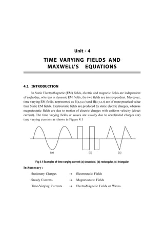
1. Unit - 4
TIME VARYING FIELDS AND
MAXWELL’S EQUATIONS
4.1 INTRODUCTION
In Static ElectroMagnetic (EM) fields, electric and magnetic fields are independent
of eachother, whereas in dynamic EM fields, the two fields are interdependent. Moreover,
time varying EM fields, represented as E(x,y,z,t) and H(x,y,z,t) are of more practical value
than Static EM fields. Electrostatic fields are produced by static electric charges, whereas
magnetostatic fields are due to motion of electric charges with uniform velocity (direct
current). The time varying fields or waves are usually due to accelerated charges (or)
time varying currents as shown in Figure 4.1
Fig 4.1 Examples of time varying current (a) sinusoidal, (b) rectangular, (c) triangular
In Summary :
Stationary Charges  Electrostatic Fields
Steady Currents  Magnetostatic Fields
Time-Varying Currents  ElectroMagnetic Fields or Waves.
(a) (b) (c)

2. Electromagnetic Fields
4.2
Table 4.1 Fundamental Relations for Electro Static and Magneto Static Model
Fundamental Relations Electrostatic Model Magnetostatic Model
Governing Equations   E = 0  . B = 0
 . D = v
  H = J
Constitutive Relations D = E
1
H B


Two major concepts are involved in this Chapter, (i) Electromotive force based on
Faradays experiments and (ii) Displacement current, which resulted from Maxwell’s
hypothesis. As a result of these concepts, Maxwell’s equations are obtained and boundary
conditions are derived for time varying fields.
4.2 FARADAY’S LAW OF INDUCTION
According to Faraday’s experiment, a static magnetic field produces no current
flow, but a time varying field produces an induced voltage called electromotive force
(emf) in a closed circuit which causes a flow of current. An electromotive force is merely
a voltage that arises from conductors moving in a magnetic field (or) from changing
magnetic fields.
Statement : The induced emf in any closed path or circuit is equal to the time rate of
change of magnetic flux linkage by the circuit. This is called as Faraday’s Law and is
expressed as:
emf
d
V
dt

  Volts (or) emf
d
V N
dt

  Volts ..............(4.1)
N denotes the number of turns of a filamentary conductor forming the closed path
and  is the flux passing through each turn. The minus sign indicates that the induced emf
is in such a direction as to produce a current whose flux if added to the original flux,
would reduce the magnitude of the emf. This is known as Lenz’s law. In other words, the
induced voltage acts in such a way as to oppose the flux producing it.
A non-zero value of
d
dt

may result from any of the following situations.
i) A time changing flux linking a stationary closed path.
ii) A time varying loop (Moving conductor) in a static magnetic field B


.
iii) A time varying loop in a time varying Magnetic field B


.

3. Time Varying Fields and Maxwell’s Equations 4.3
4.2.1 Transformer Electromotive force (Stationary Loop in a Time Vary-
ing Magnetic Field B)
Fig 4.2 A stationary closed path in a time varying B field
A stationary closed path (or) conducting loop in a time varying magnetic field B


is
shown in Figure 4.2. This emf induced by the time varying magnetic field in a stationary
loop is often referred to as transformer emf in power analysis, since it is due to transformer
action.
Electromotive force (EMF) is measured in voltage and is a scalar. It is represented
as a line integral of the electric field around a closed path.
.
emf
L
V E dl
 
 

 ...............(4.2)
The total flux through a closed circuit is equal to the integral of the normal
component of the magnetic flux density B


over the surface given by Gauss law.
.
S
B ds
  


 

 ...............(4.3)
According to Faraday’s law
emf
d
V
dt


 ...............(4.4)
Using (4.2) in equation (4.4)
emf
L
d
V E dl
dt


  

 

 ...............(4.5)
Stationary loop
I
Time varying
B field

4. Electromagnetic Fields
4.4
Using (4.3) in equation (4.5)
emf
L S
d
V E dl B ds
dt

   
 
 
 
 

 ...............(4.6)
where Vemf
is the transformer EMF.
If the circuit is stationary, and Magnetic field B is varying with time, the above
equation is rewritten as,
emf
L S
B
V E dl ds
t

    

 
 

 ...............(4.7)
The above equation is the Maxwell’s second equation in integral form. It states
that the electromotive force around a closed path is equal to the negative of the integral
of the time rate of change of magnetic flux density over the surface bounded by the
closed path.
By applying Stokes theorem to the left hand side of equation 4.7, the above equation
is rewritten as
 
S S
B
E ds ds
t

   

 


 
 

 ...............(4.8)
Stokes theorem  
L S
E dl E ds
  
 
 
  

 
For the two integrals to be equal, their integrands must be equal; that is
B
E
t

  




...............(4.9)
This equation is the point or differential form of Maxwell’s second equation. In
time varying situation, equations 4.7 and 4.9 prove that both electric and magnetic fields
are present and are inter-related. They also imply that the workdone in moving a charge
about a closed path in a time varying electric field is due to the energy from time varying
magnetic field.
4.2.2 Motional Electromotive Force (or) Moving Loop in a Static Mag-
netic Field
When a conducting loop is moving in a static magnetic field (B), and emf is induced
in the loop.

5. Time Varying Fields and Maxwell’s Equations 4.5
Fig 4.3 A closed loop moving with a velocity v in a static B field.
The force on a charge Q moving with a velocity v in a magnetic field B is given by,
F Qv B
 
 

...............(4.10)
F
v B
Q
 
 

...............(1.11)
The sliding conducting bar is composed of positive and negative charges, and each
experiences this force. The force per unit charge is called the Motional Electric Field
intensity Em
,
m
E v B
 
  

...............(4.12)
The motinal emf produced by the moving conductor is then given by
 
emf m
L L
V E dl v B dl
    
 
 

  ...............(4.13)
The other name of motional emf is flux cutting emf because it is due to the motion
action. It is the kind of emf found in electrical machines such as motors, generators and
alternators.
Consider a rod to be moving with a velocity v between a pair of rails as shown in
Figure 4.2. If the velocity v

and the magnetic field B


are mutually perpendicular to each
other, then the induced emf is given by,
 
emf
d
V v B dl vBdx vBd

     
 
 

  ...............(4.14)
where d is the length of the conductor or rod.
B
y
v
x
x=d
V
1
2
V = –B d
12 v

6. Electromagnetic Fields
4.6
Applying Stokes theorem to equation (4.13),
   
m
S S
E ds v B ds
    
 
  

...............(4.15)
(or)
 
m
E v B
   
  

...............(4.16)
4.2.3 Moving Loop in a Time Varying Magnetic Field B

In this general case of a moving conducting loop in a time varying magnetic field,
both transformer emf and the motional emf are present. Combining equations (4.7) and
(4.13) gives the total emf as,
 
.
emf
L S L
B
V E dl ds v B dl
t

      

  



  
 

  ...............(4.17)
Applying Stokes theorem
   
emf
S S S
B
V E ds ds v B ds
t

        

  


  

  ...............(4.18)
 
B
E v B
t

      



  

The above equation can also be obtained from equations (4.9) and (4.6)
4.3 DISPLACEMENT CURRENT
The point form of Ampere’s Circuital Law as it applies to steady state magnetic
fields is given by
H J
 

 

...............(4.19)
It is inadequate for time varying conditions. Taking divergence of equation (4.19)
  0
H J
     ...............(4.20)
Since the divergence of a Curl is zero, . J is also zero. However, according to the
equation of continuity

7. Time Varying Fields and Maxwell’s Equations 4.7
.
v
J
t


  

...............(4.21)
For equation (4.20) to be true,
v
t



has to be zero. This is an unrealistic limitation
and hence equation (4.19) has to amended for time varying fields.
Hence D
H J J
  

 
 

...............(4.22)
Taking Divergence,
  D
H J J
     

 
 

0 v
D
J
t


  

v
D
J
t


 

...............(4.23)
Replacing v
by .D (Point form of Gauss Law)
 
D
D
J D
t t
 
    
 
...............(4.24)
D
D
J
t



D
t


is the displacement current density in A/m2
. Ampere’s circuital law in point
form (substituting eqn. 4.24 in 4.22) becomes
D
H J
t

  

...............(4.25)
where J represents conduction current density and
D
t


is the displacement current
density. Equation (4.25) is the Maxwell’s 1st equation in point or differential form
based on Ampere’s circuital law for time varying fields.
Integrating both sides of equation (4.25)

8. Electromagnetic Fields
4.8
 
S S S
D
H ds J ds ds
t

     

  


...............(4.26)
Rewriting the above equation by applying Stokes theorem to L.H.S. results in
S
D
H dl J ds ds
t

    

  
 
S
D
H dl J ds
t

 
   
 

 
 
 ...............(4.27)
This is the integral form of Maxwell’s 1st equation from Amperes circuital law.
It is stated as follows,
The line integral of Magnetic field intensity around a closed path is equal to
the integral of sum of conduction current density and displacement current density
over the surface bounded by the closed path.
4.4 MAXWELL’S EQUATION FROM GAUSS’S LAW
Gauss law states that electric flux passing through any closed surface is equal to
the total charge enclosed by the surface.
enc
D ds Q
 

 

...............(4.28)
where,
Vol
enc v
Q dv

  is the volume charge density. Hence equation (4.28) can be
rewritten as
v
v
D ds dv

 
 
 

...............(4.29)
The above equation is the integral form of Maxwell’s equation for electric fields
derived from Gauss’s law.
Applying the divergence theorem for the L.H.S. of equation (4.29)
 
.
S V
D ds D dv
 
  ...............(4.30)
Using equation (4.30) in (4.29), the equation becomes

9. Time Varying Fields and Maxwell’s Equations 4.9
 
. v
V V
D dv dv

 
  ...............(4.31)
Assuming same volume for integration on both sides.
.D = v
...............(4.32)
The above equation is the point or differential form of Maxwell’s equation for
electric fields derived from Gauss’s Law.
Magnetic flux lines are closed and do not terminate on a charge. Hence the surface
integral of B over a closed surface is zero, since there is no magnetic charge. The Gauss
law for magnetic field is
0
S
B ds
 
 ...............(4.33)
This is the integral form of Maxwell’s equation for Magnetic fields derived
from Gauss’s Law.
Using Divergence theorem, the surface integral can be converted into volume integral
 
. 0
V
B dv
 
 ...............(4.34)
Hence for a finite volume,
.B = 0 ...............(4.35)
This is the differential form or point form of Maxwell’s equation for Magnetic
fields derived from Gauss’s Law.
4.5 MAXWELL’S EQUATIONS IN POINT OR DIFFERENTIAL FORM
Electromagnetic fields in their time varying form constitute electromagnetic waves
(EM waves). These Electromagnetic fields/ waves are useful in all communication and
radar systems. The electric and magnetic fields of the EM waves are related through the
Maxwell’s equations.
Maxwell’s equations describe the inherent properties of the field vectors and their
relationships. They form the starting point for the solutions of many problems and have
numerous applications. They are also referred as Electromagnetic field equations.
Maxwell’s equations are four expressions derived from Ampere’s circuital law,
Faraday’s law, Gauss law for electric field and Gauss law for magnetic field.

10. Electromagnetic Fields
4.10
i) Maxwell’s equation from Ampere’s Circuital law.
D
H J
t

  

...............(4.36)
ii) Maxwell’s equation from Faraday’s law
B
E
t

  

...............(4.37)
iii) Maxwell’s equation from Gauss law for Electric fields.
V
D 
  ...............(4.38)
iv) Maxwell’s equation from Gauss law for Magnetic fields.
0
B
   ...............(4.39)
The above four partial differential equations relate the electric and magnetic fields
to each other and to their sources, charge and charge density.
The following auxillary equations are required to define and relate the quantities
appearing in Maxwell’s equation.
i) D = E ...............(4.40)
ii) B = H ...............(4.41)
iii) J = E (Conduction current density) ...............(4.42)
iv) J = V
v (Convection current density) ...............(4.43)
where H  Magnetic field intensity (A/m)
E  Electric field intensity (V/m)
J  Conduction current density (A/m2
)
B  Magnetic flux density (Wb/m2
or Tesla)
V
 Volume charge density (C/m2
)
D  Electric flux density (C/m2
)
4.6 MAXWELL’S EQUATION IN INTEGRAL FORM
The integral forms of Maxwell’s equations are usually easier to recognize in terms
of the experimental laws from which they have been obtained by a generalization process.

11. Time Varying Fields and Maxwell’s Equations 4.11
i) From Ampere’s Circuital Law:
Taking surface integral on both sides of equation (4.36)
  .
s S S
D
H ds J ds ds
t

    

   ..............(4.44)
Applying the Stokes theorem to the LHS, the above equation is rewritten as
L S
D
H dl J ds
t

 
   
 

 
 
 ..............(4.45)
ii) From Faraday’s Law :
Taking surface integral of equation (4.37) on both sides.
 
S S
B
E ds ds
t

   

  ..............(4.46)
Applying Stokes theorem to the LHS of the above equation
 
S L
E ds E dl
   
 
 ..............(4.47)
Equation (4.46) is rewritten as
L S
B
E dl ds
t

   

 
 ..............(4.48)
iii) From Gauss Law for Electric Fields :
Taking volume integral on both sides of equation (4.38)
 
V V
v
D dv dv

 
  ..............(4.49)
Applying Divergence theorem,
 
V
S
D ds D dv
  
 
 ..............(4.50)
Substituting (4.50) in (4.49),
v
S v
D ds dv Q

  
 
 ..............(4.51)

12. Electromagnetic Fields
4.12
iv) From Gauss Law for Magnetic Fields:
Taking volume integral of equation (4.39)
  0
v
B dv
 
 ..............(4.52)
Applying divergence theorem to LHS of (4.52)
 
.
S
v
D dv B ds
  
 
 ..............(4.53)
Hence 0
S
B ds
 

 ..............(4.54)
Equations (4.45), (4.48), (4.51) and (4.54) are Maxwell equations in integral form.
These four integral equations enable us to find the boundary conditions on B, D, H and E
which are necessary to evaluate the constants obtained in solving the Maxwell’s equations
in partial differential form.
4.7 TIME HARMONIC (SINUSOIDAL) FIELDS
A time harmonic field is one that varies periodicallyor sinusoidallywithtime. Sinusoidal
analysis is of practical value and can be extended to most waveforms by Fourier Analysis.
Sinusoids are easily expressed in phasors, which are more convenient to work with.
A phasor is a complex number that contains the amplitude and phase of a sinusoidal
oscillation. As a complex number, a phasor z can be represented as
z = x + jy = r  ..................(4.55)
(or) z = r ej
= r(cos+jsin) ..................(4.56)
where 1,
j x
  is the real part of z, y is the imaginary part of z, r is the magnitude of z
which is given by
2 2
| |
r z x y
   ..................(4.57)
and  is the phase of z given by
1
tan /
y x
 
 ..................(4.58)
The phasor z can be represented in rectangular form as z = x + jy or in polar form as
z = r = r ej
. Addition and subtraction of phasors are better performed in rectangular
form. Multiplication and division are better done in polar form.

13. Time Varying Fields and Maxwell’s Equations 4.13
To introduce a time element, let
 = t +  ..................(4.59)
where may be a function of time or space co-ordinate or a constant. Then
rej
= rej
. ejt
..................(4.60)
The real part of rej
is given by
Re(rej
) = r cos(t + ) ..................(4.61)
and the imaginary part of rej
is given by
Im(rej
) = r sin (t + ) ..................(4.62)
Let the applied Electric field be denoted as
E(t) = E0
cos (t + ) = Re[E0
ej
. ejt
] ..................(4.63)
where E0
= Magnitude (or) Amplitude
 = Angular frequency
= Phase angle
The above equation equals the real part of E0
ej
. ejt
The complex term E0
ej
which results from dropping the time factor in E(t), is
called Phasor Electric field and is denoted by ES
.
ES
= E0
ej
= E0
 ..................(4.64)
where the subscript s denotes the phasor form of E(t). Thus the instantaneous form E(t)
=E0
cos(t + ) can be expressed as
E(t) = Re(ES
. ejt
) ..................(4.65)
In general, if a vector A(x, y, z, t) is a time harmonic field, the phasor form of A is
AS
(x, y, z); the two quantities are related by
A = Re(AS
ejt
) ..................(4.66)
4.8 MAXWELL’S EQUATION IN PHASOR FORM / TIME HARMONIC
MAXWELL’S EQUATIONS FOR HARMONICALLY VARYING FIELDS
The electric flux density that is varying harmonically with time is given by
0
j t
D D e 


..................(4.67)

14. Electromagnetic Fields
4.14
The Magnetic flux density is also written as
0
j t
B B e 



..................(4.68)
Taking partial derivative of the above equations results in
0
j t
D
j D e j D
t

 

 



..................(4.69)
0
j t
B
j B e j B
t

 

 





..................(4.70)
Phasor Form of Maxwell’s Differential (or) Point Form Equations :
Using the above equations, the Maxwell’s equations are rewritten as,
i)
D
H J E j D E j E
t
   

      

   
..................(4.71)
 
H j E
 
  

 
 From Ampere’s law
ii)
B
E j B j H
t
 

      


 

..................(4.72)
E j H

 
 

 From Faraday’s law
iii)  . D = V
 From Gauss law for Electric fields ..................(4.73)
iv)  . B = 0  From Gauss for Magnetic fields ..................(4.74)
Phasor Form of Maxwell’s Integral Equations :
Using Equations (4.69) and (4.70), the general Maxwell’s equations are rewritten
as
(i)  
S S
D
H dl J ds E j D ds
t
 

 
    
 

 
  
 
   
S S
E j E ds j E ds
   
    
 
 
S
H dl j E ds
 
   
 
  From Ampere’s law ..................(4.75)

15. Time Varying Fields and Maxwell’s Equations 4.15
(ii)
S S
B
E dl ds j B ds
t


      

  

s
j H ds

  

S
E dl j H ds

   
 
  From Faraday’s law ..................(4.76)
iii)
V
V
v
S
D ds d

 
 
  From Gauss Law for Electric fields ..................(4.77)
iv) 0
S
B ds
 

  From Gauss Law for Magnetic fields ..................(1.78)
4.9 ELECTROMAGNETIC BOUNDARY CONDITIONS (OR) MAXWELL’S
EQUATIONS AND BOUNDARY CONDITIONS
Boundary conditions are derived by applying the integral form of Maxwell’s
equations to a small region at an interface of two media in a manner similar to that used
in obtaining the boundary conditions for static electric and magnetic fields.
In general, the application of the integral form of a curl equation to a flat closed
path at a boundary with top and bottom sides in the two touching media yields the boundary
condition for the tangenital components and the application of the integral form of a
divergence equation to a shallow pill box at an interface with top and bottom faces in the
two contiguous media gives the boundary condition for the normal components.
Boundary Conditions for Electric Fields :
Consider the E field existing in a region that consists of two different dielectrics
characterised by 1
and 2
. The fields E1
and E2
in media 1 and media 2 can be decomposed
as
E1
= Et1
+ En1
E2
= Et2
+ En2
..................(4.79)

16. Electromagnetic Fields
4.16
Fig 4.4 Electric boundary conditions
Consider the closed path abcda shown in Figure 4.4. By conservative property
0
E dl
 

 ..................(4.80)
0
b c d a
a b c d
E dl E dl E dl E dl
       
    ..................(4.81)
1 1 2 2 2 1 0
2 2 2 2
t n n t n n
h h h h
E E E E E E
 
   
       
Et1
 – Et2
 = 0
(Et1
– Et2
)  = 0  Et1
– Et2
= 0,   0
Et1
= Et2
..................(4.82)
The tangenital components of Electric field intensity are continuous across the
boundary.
In vector form  
1 2 0
n t t
a E E
  

  

..................(4.83)
Since D = E, equation (4.82) can be written as
1 2
1 2
t t
D D
 
 ..................(4.84)
1 1
2 2
t
t
D
D


 ..................(4.85)
Dn1
D1
Dt1
Dn2
D2
Dt2
Dn1
s
h
a
d c
h
 b
En1
E1
Et1
En2
E2
Et2

17. Time Varying Fields and Maxwell’s Equations 4.17
Consider a cylindrical Gaussian Surface (Pill box) shown in the Figure 4.4, with
height h and with top and bottom surface areas as s.
By Gauss law,
S
D ds Q
 

 ..................(4.86)
Top Bottom sides
0
D ds D ds D ds
     
   ..................(4.87)
The Electric flux through the sides is zero
sides
0
D ds
 

Hence equation (4.87) becomes,
Dn1
s – Dn2
s =Q=S
s ..................(4.88)
where S
is the surface free charge density
Dn1
– Dn2
= S
..................(4.89)
In vector form
 
1 2
n n n S
a D D 
  

 
 
..................(4.90)
For a perfect dielectric S
= 0. Equation (4.89) is rewritten as
Dn1
– Dn2
= 0
Dn1
= Dn2
..................(4.90(a))
The normal components of the electric flux density are continuous across the
boundary if there is no free surface charge density.
Since D = E, Equation (4.90(a)) is rewritten as
1
En1
= 2
En2
..................(4.91)
1 2
2 1
n
n
E
E


 ..................(4.92)
Magnetic Boundary Conditions :
Consider a magnetic boundary formed by two isotropic homogenous linear materials
with permeability 1
and 2
.

18. Electromagnetic Fields
4.18
Fig 4.5 Magnetic boundary conditions
Consider a small cylindrical gaussian surface of length h, with top and bottom
surfaces areas s as shown in Figure 4.5. Applying the Gauss law for magnetic field
0
S
B ds
 

 ..................(4.93)
Bn1
s–Bn2
s = 0, Bn1
– Bn2
= 0
Bn1
= Bn2
..................(4.94)
In vector form
 
1 2 0
n n n
a B B
  

 
 

..................(4.95)
The normal components of magnetic flux density is continuous across the boundary.
Since B = H, equation(4.94) can be rewritten as
1
Hn1
= 2
Hn2
1 2
1 1
n
n
H
H


 ..................(4.96)
Consider a closed path abcda of length  and height h. Applying Ampere’s
circuital law
H dl I
 

 ..................(4.97)
. . . .
b
a b c d
c d a
H dl H dl H dl H dl I
   
   
   ..................(4.98)
Bn1
B1
Bt1
Bn2
B2
Bt2
Bn1
s
h
a
d c
h
 b
Hn1
H1
Ht1
Hn2
H2
Ht2

19. Time Varying Fields and Maxwell’s Equations 4.19
1 1 2 2 1 2 2
2 2 2
t n n t n n
h h h
H H H H H h H
 
  
       
Ht1
 – Ht2
 = I
(Ht1
– Ht2
)  = I
1 2
1
t t s
H H J

  

..................(4.99)
where Js
, is the surface current density. The tangenital components of the Magnetic field
intensity H


are discontinuous at the boundary where a free surface current exists.
In vector form,  
1 2 ( / )
n t t S
a H H J A m
  


..................(4.100)
where n
a


is the unit vector normal to the interface and is directed from medium 1 to
medium 2.
Since B =  H. equation (4.99) can be written as
1 2
1 2
t t
s
B B
J
 
  ..................(4.101)
Electromagnetic Boundary Condition : General Statements
i) The tangenital component of an E field is continuous across an interface
Et1
= Et2
(V/m) ..................(4.102)
ii) The tangenital component of an H field is discontinous across an interface where a
surface current exists
Ht1
– Ht2
= Js
(A/m) ..................(4.103)
iii) The normal component of D field is discontinuous across an interface where surface
charge density exists.
Dn1
– Dn2
= s
(C/m2
) ..................(4.104)
iv) The normal of a B field is continuous across an interface
Bn1
= Bn2
(Tesla) ..................(4.105)

20. Electromagnetic Fields
4.20
4.10 POTENTIAL FUNCTIONS/THE RETARTED POTENTIALS
Wave equation for vector potential  
A

Magnetic flux density B and Vector magnetic potential (A) are related by the
following equations
B A
 


Tesla ...............(4.106)
From Faraday’s law,  
B
E A
t t
 
     
 



  0
E A
t

   

 
...............(4.107)
0
A
E
t

   




0
A
E
t
 

  
 

 



The two vector quantities inside the brakcet are curl free and hence can be expressed
as gradient of a scalar. From the definition of electric scalar potential.
A
E V
t

  




A
E V
t

  




...............(4.108)
For static fields 0
A
t





, and E V
 

For static field E is determined team valone and for time varying fields E depends
on both V and A. The electric field of equation (4.108) consists of two parts.
(i) –V due to charge distribution V
(ii)
A
t


is due to time varying current J

21. Time Varying Fields and Maxwell’s Equations 4.21
The scalar electric potential V and Magnetic Vector potential A

are given by
0 V
1
4
v
V dv
R


  ...............(4.109)
0
V
4
J
A dv
R


 

...............(4.110)
When V
and J vary slowly with time and the range R is small then substituting
(4.106) and (4.108) in the following equation
D
H J
t

  



X by  on both sides
E
H J
t
  

  



A
J V
t t
 
 
 
   
 
 
 
...............(4.111)
A
B J V
t t
 
 
 
    
 
 
 


...............(4.112)
  A
A J V
t t
 
 
 
     
 
 
 




Vector identity
  2
A A A
     

 

 
2
2
2
V A
A A J
t t
  
 
 
      
 
 
 

...............(4.113)
 
2
2
2
A V
A A J
t t
  
 
 
        
 
 



22. Electromagnetic Fields
4.22
2
2
2
.
A V
A J A
t t
  
 
 
       
 
 
 

...............(4.114)
Let . 0
V
A
t


  



...............(4.115)
2
2
2
A
A J
t
 

   

...............(4.116)
Equation (4.116) is the non homogenous wave equation for vector potential A. It
is called wave equation because the solutions represents waves travellng with a velocity
equal to 1  .
Equation (4.115) is called the Lorentz condition for potential. For static fields
Lorentz condition is 0
A
 


.
Wave equation for Scalar Potential (V)
Substituting equation (4.108) in the following equation
.D = V
.E = V
V
V
A
t
 

 
   
 

 
V
V
A
t




 
   
 

 
 
2 V
V A
t




   



...............(4.117)
From Lorentz condition equation (4.115)
V
A
t


  


...............(4.118)
Sub (4.113) in (4.117) yields
2 V
V
V
t t




 
 
   
 
 
 
...............(4.119)

23. Time Varying Fields and Maxwell’s Equations 4.23
2
2 V
2
V
V
t





  

...............(4.120)
Equation (4.120) is the non homogenous wave equation for scalar potential V.
The soltuions to equations (4.116) and (4.120) are
 
 
Wb/m
4
V
J dV
A
R


  ...............(4.121)
and
 
 
V
V
4
dV
V V
R


  ...............(4.122)
The terms [V
] or [J] means that the time t in V
(x, y, z, t) or J(x, y, z, t) is replaced
by a retarded time t given by
1 R
t t
u
  ...............(4.123)
Where R = |r–r| is the distance between the source point r and the observation
point r and
1
u


Where u is the velocity of propagation. In free space, u = c = 3  108
m/s is the
speed of light is Vacuum.
Potentials V and A are called the retarted electric scalar potential and retarted
magnetic vector potential. The use of retarted time has resulted in time varying potentials
known as retarted potentials.
4.11 WAVE EQUATIONS AND THEIR SOLUTION
Wave :
If a physical phenomenon that occurs at one place at a given time is reproduced at
other places at later times, the time delay being proportional to the space seperation from
the first location, then the group of phenomena constitute a wave.
In general, Waves are means of transporting energy or information.
A wave is a carrier of energy or information and is a function of both time and
space. Typical examples of Electro Magnetic (EM) waves include radio waves, TV signals,
radar beams and light rays. All forms of EM energy share three fundamental characteristics:

24. Electromagnetic Fields
4.24
(i) They all travel with high velocity;
(ii) In traveling, they assume all the properties of waves; and
(iii) They radiate outward from a source.
Maxwell predicted the existence of EM waves and established it through well known
Maxwell’s equations. The same EM waves were investigated by Heinrich Hertz. Hertz
conducted several experiments on EM waves and he succeeded in generating and detecting
radio waves. These radio waves are also called Hertzian waves.
Applications of EM waves:
(i) They have a wide range of applications in all types of communications like
Television, satellite, wireless, cellular and mobile communications etc.
(ii) EM waves are also used in radiation therapy and microwave ovens etc.
(iii) In all types of radars like doppler radar, airport surveillance radar, weather
forcasting radar, remote sensing radar etc.
The major goal is to solve Maxwell’s equations and describe EM wave motion in
the following media:
(1) Free space ( = 0, = 0
,  = 0
)
(2) Lossless dielectrics (= 0, =r
0
, =r
0
(or) <<)
(3) Lossy dielectrics (0, =r
0
, =r
0
)
(4) Good conductor (  , =0
, =r
0
(or)  >>)
Where  is the conductivity of the medium,
 is the permittivity of the medium
 is the permeability of the medium
 is the angular frequency of the wave.
A homogenous medium is one for which the quantities ,  and  are constnat
throughout the medium. The medium is isotropic it  is constant, so that D and E have
come direction everywhere.
4.11.1 Wave Propagation in free space : (source free wave equations)
Consider an electomagnetic wave propagating through free space. The medium
(free space) is sourceless - ie., V
= 0. Free space contains no charges and hence no
conduction current. ie  = 0, J=E = 0.

25. Time Varying Fields and Maxwell’s Equations 4.25
For free space the Maxwell’s equations are as follows:
(i) 0
D E
H
t t

 
  
 
(J = 0 for free space) ...............(4.124)
(ii) 0
B H
E
t t

 
    
 
...............(4.125)
(iii) . D = 0 as V
= 0 for free space ...............(4.125a)
(iv)  . B = 0 ...............(4.125b)
Wave equation for Electric field
Differentiating equation (4.124) with respect to time
 
2
0 2
E
H
t t

 
 
 
...............(4.126)
 operator indicates differentiation with respect to space while
t


indicates
differentiation with respect to time. Both are independent of each other and hence the
operators can be interchanged.
Equation (4.126) is rewritten as
2
0 2
H E
t t

 
 
 
...............(4.127)
Taking the curl of equation 4.125,
0
H
E
t


  

...............(4.128)
From vector identity
  2
.
E E E
       ...............(4.129)
Equation (4.128) and (4.129)
  2
0 0
.
H H
E E
t t
 
 
 
        
 
 
 
...............(4.130)
Substituting (4.126) in (4.130)

26. Electromagnetic Fields
4.26
 
2 2
2
0 0 0 0
2 2
.
E E
E E
t t
   
 
 
      
 
 
 
...............(4.131)
From equation (4.125a), 0
D
 
0 0
E

 
0
E
  since 0
 0 ...............(4.132)
Substituting (4.132) in (4.131)
2
2
0 0 2
E
E
t
 

  

2
2
0 0 2
E
E
t
 

 

...............(4.133)
This is the wave equation for a time varying electric field in free space conditions.
Wave equation for Magnetic field :
Taking time derivative of equation (4.125)
 
2
0 2
H
E
t t

 
  
 
...............(4.134)
Since the cul operation is differentiation with respect to space, the order of
differentiation may be reversed.
2
0 2
E H
t t

 
  
 
...............(4.135)
Taking curl of equation (4.124)
0
E
H
t


  

...............(4.136)
From vector identity
  2
.
H H H
       ...............(4.137)
Equation (4.137) and (4.136) gives

27. Time Varying Fields and Maxwell’s Equations 4.27
  2
0
.
E
H H
t


    

  2
0
.
E
H H
t


 
    
 

 
...............(4.138)
Substituting (4.135) in (4.138) yields
 
2
2
0 0 2
.
H
H H
t
 
 

    
 

 
 
2
2
0 0 2
.
H
H H
t
 

     

...............(4.139)
From equation (4.125b), . B = 0
 . 0
H = 0
. H = 0 since   0 ...............(4.140)
Substituting (4.140) in (4.139) gives
2
2
0 0 2
H
H
t
 

  

2
2
0 0 2
H
H
t
 

 

...............(4.141)
This is the wave equation for time varying magnetic field in free space.
The wave equations (4.133) and (4.141) can be rewritten as
2
2
0 0 2
0
E
E
t
 

  

(or)
2
2
2 2
1
0
E
E
u t

  

...............(4.142)
2
2
0 0 2
0
H
H
t
 

  

(or)
2
2
2 2
1
0
H
H
u t

  

...............(4.143)
Where 8
0 0
1 3 10 /
u m s
 
   = Velocity of Propagation
Equations (4.142) and (4.143) are called homogenous vector wave equations

28. Electromagnetic Fields
4.28
Using time harmonic Maxwells equations,
E = –jH, H jE, . E = 0, . H = 0 and
2 2
2 2 2 2
2 2
, , ,
E H E H
j E j H j E j H
t t t t
   
   
   
   
Equations (4.142) and (4.143) can be rewritten as
2
2
2
0
E E
u

   2
E + K2
E = 0 ...............(4.144)
2
2
2
0
H H
u

   2
H + K2
H = 0 ...............(4.145)
Where, K
u

 is the wave number. Equations (4.144) and (4.145) are homogenous
vector Helmholtzs equations.
4.12 TIME HARMONIC ELECTROMAGNETICS
Field vectors that vary with space coordinates and are sinusoidal functions of time
can be represented by vector phasors that depend on space coordinates but not on time.
As an example, a time harmonic E field referring to coswt can be written as
E(x, y, z, t) = Re[E(x, y, z) ejt
]
Where E(x, y, z) is a vector phasor that contains information on direction, magnitude
and phase. Phasors are in general complex quantities.
Time harmonic Maxwell equations in terms of vector phasors (E, H) and source
phasors (, J) in a simple (linear, isotropic and homogenous) medium are given as follows:
  E = –jH ...............(4.146)
  H = J + jE ...............(4.147)
. D = V
(or) . V
E


  ...............(4.148)
. B = 0 (or) .H = 0 ...............(4.149)
The wave equation for vector potential is given by equation 4.116 as,

29. Time Varying Fields and Maxwell’s Equations 4.29
2
2
2
A
A J
t
 

   

...............(4.150)
In phasors,
A
j A
t




and
2
2 2
2
A
j A
t




...............(4.151)
Substituting equation (4.151) in equation (4.150)
 
2 2 2
A j A J
  
    
2
A + 2
A = –j
2
2
2
A A J
u


    , where u is the velocity of propagation
2
A + K2
A = –j ...............(4.152)
Where K
u

 
  and is called as the wave number.
.
Similarly the wave equation for scalar potential is given by equation 4.120 as,
2
2
2
V
V
V
t




   

...............(4.153)
 
2 2 2 V
V j V

 

   
2
2
2
V
V V
u



   
2 2 V
V K V


    ...............(4.154)
Equations (4.152) and (4.153) are called as non homogenous Helmholtz’s equations.
The Lorentz condition for potentials is given by
0
V
A
t


  

...............(4.155)
In terms of phasors, the above equation is written as

30. Electromagnetic Fields
4.30
.A + (jV) = 0 ...............(4.156)
The phasor solutions for equation (4.152) and (4.153) are given as
1
4
jKR
V
V
e
V dv
R



  ...............(4.157)
4
jKR
V
Je
A dv
R



  ...............(4.158)
These are the expressions for retarded scalar and vector potentials due to time
harmonic sources.
Taylor series expansion for the exponential factor e–jKR
is
2 2
1 .....
2
jKR K R
e jKR

    ...............(4.159)
where K
u

 = wave number. K can be defined in terms of wavelength
u
f
  in
the medium and is expressed as
2 2 2
f u
K
u u u
   
 
 
   
 
 
...............(4.160)
Thus if 2 1
R
KR 

  ...............(4.161)
or if the distance R is very small in camparison to the wavelength , e–jKR
can be
approximated by 1.
Equation (4.157) and (4.158) then simplify to static expressions as
1
4
V
V
V dv
R


  ...............(4.161a)
4 V
J
A dv
R


  ...............(4.161b)
The formal procedure for finding the electric and magnetic fields due to time
harmonic charge and current distribution is as follows:

31. Time Varying Fields and Maxwell’s Equations 4.31
(i) Find phasors V and A from equations (4.157) and (4.158)
(ii) Find phasors E = –V–jA and B = A
(iii) Find the instantaneous E(R, t) = Re
[E(R)ejt
] and B(R, t) = Re
[B(R) ejt
] for a
cosine reference.
4.13 THE ELECTROMAGNETIC SPECTRUM
The electromagnetic spectrum is the range of frequencies of electromagnetic
raditation and their respective wavelengths and photon energies. It covers electromagnetic
waves with frequencies ranging from below one Hertz to above 1025
Hertz, corresponding
to wavelengths from thousands of kilometers down to a fraction of the size of an nucleus.
It extends from very low power frequencies through radio, television, microwave,
infrared, visible light, ultra violet, X-ray and Gamma () ray frequencies exceeding 1024
Hz. All electromagnetic waves in whatever frequency range propagate in a medium with
same velocity, u=1  (u=C=3108
m/s in air). Figure 4.6 shows the electromagnetic
spectrum divided in to frequency and wavelength ranges on logarthmic scales according
to application and natural occurance. The term “microwave” denotes electromagnetic
waves above a frequency of 1 GHz and all the way upto the lower limit of the infrared
band, encompassing, UHF, SHF, EHF and mm-wave regions.

32. Electromagnetic Fields
4.32
Fig.4.6 Spectrum of electromagnetic waves
Wavelngth
(m)

Frequency
(Hz)
f
Application
and Classification
Photo Energy
(eV)
hf
(GeV)
(MeV)
(keV)
(eV)
(meV) 10
–3
1
10
3
10
6
10
9
10
24
10
–15
-rays
X-rays
Ultraviolet
10
21
10
18
(EHz)
10
15
(PHz)
10
12
(THz)
visible light
Infrared
mm wave
EHF (30–300 GHz) Radar
Radar, satellite
communication
Radar, TV, navigation
TV, FM, police, mobile
radio, air traffic control
Facsimile, SW radio,
citizen’s band
AM, maritime radio,
direction finding
Navigation,
radio beacon
Navitation, sonar
SHF (3–30 GHz)
UHF (300–3000 MHz)
UHF (300–300 MHz)
HF (3–30 MHz)
MF (300–3000 kHz)
LF (30–300 kHz)
VLF (3–30 kHz)
ULF (300–3000 Hz)
SLF (30–300 Hz)
ELF (3–30 Hz)
10
9
(GHz)
10
6
(MHz)
–60 (Hz)
10
3
(kHz)
1 (Hz)
10
–12
10
–10
10
–19
10
–6
10
–3
10
–2
10
–1
(m) 1
10
10
2
10
3
10
4
10
5
10
6
10
7
10
8
(Mm)
(km)
(cm)
(mm)
( m)

(nm)
(A)