The document presents various outlier detection methods categorized into probabilistic-based, proximity-based, linear models, outlier ensembles, and neural networks. It discusses techniques such as angle-based outlier detection, local outlier factor, one-class support vector machines, and isolation forest, detailing their mechanisms and implications. Additionally, it contains a benchmark section comparing these methods' performance based on execution time and precision-recall metrics using a credit card transaction dataset.

1. 1
DaeJin Kim
Outlier Detection Method
Introduction

2. 2
Table of Contents
1. Probabilistic-based Method
1. Histogram-Based Outlier Detection
2. k Nearest Neighbors
3. Local Outlier Factor
2. Proximity-based Method
1. One-Class Support Vector Machines
2. Principal Component Analysis
3. Linear model
1. Isolation Forest
4. Outlier Ensembles
1. Angle-Based Outlier Detection 1. AutoEncoder
5. Neural Network
1. Data
2. Model Selection
3. Model Comparison
6. Benchmark

3. 3
Probabilistic-based Method
The spectrum of angles to pairs of points remains rather (1) small for an outlier whereas (2) the variance of
angles is higher for border points of a cluster and (3) very high for inner points of a cluster.
1. Angle-Based Outlier Detection (ABOD)
: The Angle-Based Outlier Factor ABOF is the variance over the angles between the difference vectors of
one point to all pairs of other points in set weighted by the distance of the points

4. 4
Probabilistic-based Method
The spectrum of angles to pairs of points remains rather (1) small for an outlier whereas (2) the variance of
angles is higher for border points of a cluster and (3) very high for inner points of a cluster.
1. Angle-Based Outlier Detection (ABOD)
: The Angle-Based Outlier Factor ABOF is the variance over the angles between the difference vectors of
one point to all pairs of other points in set weighted by the distance of the points
Outlier
Outlier

5. 5
Probabilistic-based Method
1. Angle-Based Outlier Detection (ABOD)
: The Angle-Based Outlier Factor ABOF is the variance over the angles between the difference vectors of
one point to all pairs of other points in set weighted by the distance of the points
- Angle-Based Outlier Factor
* Weighted by the distance of the points : Increase the affects of the nearby points

6. 6
Probabilistic-based Method
1. Angle-Based Outlier Detection (ABOD)
: The Angle-Based Outlier Factor ABOF is the variance over the angles between the difference vectors of
one point to all pairs of other points in set weighted by the distance of the points
- Speed-up by Approximation (used for Benchmark) : Only consider k near points
* Weighted by the distance of the points : Increase the affects of the nearby points

7. 7
Proximity-based Method
1. Histogram-Based Outlier Detection (HBOS)
: Histogram-Based Outlier Detection assumes independence. A histogram for each single feature can be
computed, scored individually and combined at the end for detect outliers.
Since it assumes independence of the features, it can be computed much faster than multivariate approaches at
the cost of less precisions.
(sqlservercentral.com)

8. 8
Proximity-based Method
1. Histogram-Based Outlier Detection (HBOS)
: Histogram-Based Outlier Detection assumes independence. A histogram for each single feature can be
computed, scored individually and combined at the end for detect outliers.
The HBOS of every instance p is calculated using the corresponding height of the bins where the instances is
located:
* Take the sum of the logarithms to get the effect of multiplication.

9. 9
Proximity-based Method
2. k Nearest Neighbors (kNN)
: Similar to classification, kNN outlier detection uses the distances to the kth nearest neighbors as the
outlier scores.
The distance is calculated by: (1) Largest value, (2) Mean value, (3) Median value

10. 10
Proximity-based Method
3. Local Outlier Factor (LOF)
: Calculate how isolated the object is with respect to the surrounding neighborhood.
Unlike other proximity-based methods, LOF considers the density difference.
Outlier
Outlier ?

11. 11
Proximity-based Method
3. Local Outlier Factor (LOF)
: Calculate how isolated the object is with respect to the surrounding neighborhood.
- Definition of LOF
1) k-distance of an object p : distance to the kth most distant point
2) reachability distance of an object p w.r.t. object o
3) local reachability density of an object p

12. 12
Proximity-based Method
3. Local Outlier Factor (LOF)
: Calculate how isolated the object is with respect to the surrounding neighborhood.
- Definition of LOF
4) Local Outlier Factor
• P is located at a low density => LOF higher
• Other points are located at a high density => LOF higher
∴ Density difference determines LOF

13. 13
Proximity-based Method
3. Local Outlier Factor (LOF)
: Calculate how isolated the object is with respect to the surrounding neighborhood.
- LOF example
𝒍𝒅𝒓 𝒌(𝑨) High Low Low
𝒍𝒅𝒓 𝒌(𝑩) High High Low
𝑳𝑶𝑭 (𝑨) Low High Low

14. 14
Linear Model
- Support Vector Machines with two classes
Search the hyperplane that has maximal margin between the classes.
* Soft Margin: To prevent the SVM classifier from overfitting with train data, slack variables 𝜉𝑖 are introduced to
allow some data points to lie within the margin.
1. One-Class Support Vector Machines (OCSVM)

15. 15
Linear Model
1. One-Class Support Vector Machines (OCSVM)
- Support Vector Machines with two classes
Search the hyperplane that has maximal margin between the classes.
* Soft Margin: To prevent the SVM classifier from overfitting with train data, slack variables 𝜉𝑖 are introduced to
allow some data points to lie within the margin.
• The objective function:
• The decision function for a data point x:
(𝛼𝑖 are the Lagrange multipliers, 𝐾 is the kernel function)
* The constant C > 0 determines the trade-off between maximizing
the margin and the number of training data points within that margin

16. 16
Linear Model
- Support Vector with One-Class
Separates all the data points from the origin in feature space F and maximizes the distance from this
hyperplane to the origin.
1. One-Class Support Vector Machines (OCSVM)

17. 17
Linear Model
- Support Vector with One-Class
Separates all the data points from the origin in feature space F and maximizes the distance from this
hyperplane to the origin.
• The objective function:
• The decision function for a data point x:
* 𝜈 ∈ (0,1) is a parameter to trade-off the smoothness of 𝑓(𝑥) and
fewer falling on the same side of the hyperplane as the origin in F.
(𝛼𝑖 are the Lagrange multipliers, 𝐾 is the kernel function)
1. One-Class Support Vector Machines (OCSVM)

18. 18
Linear Model
2. Principal Component Analysis (PCA)
: Find the principal components, and use the sum of squares of the standardized principal component
scores for the anomaly score.
PCA uses an orthogonal transformation to find a low-dimensional space that maximizes variance of converted
data.
-Principal Component Analysis
- The standardized principal component scores
* The first few principal components have large variances and explain the largest
cumulative proportion of the total sample variance.

19. 19
Outlier Ensembles
1. Isolation Forest
: Randomly generated binary trees where instances are recursively partitioned, these trees produce
noticeable shorter paths for anomalies since in the regions occupied by anomalies.
Anomalies are more susceptible to isolation and hence have short path lengths.
Outlier

20. 20
Outlier Ensembles
1. Isolation Forest
: Randomly generated binary trees where instances are recursively partitioned, these trees produce
noticeable shorter paths for anomalies since in the regions occupied by anomalies.
- The anomaly score s of an instance x:
where

21. 21
Neural Network
1. AutoEncoder
: Train AutoEncoder using train data and get anomaly score with reconstruction error of pre-trained
AutoEncoder.
-AutoEncoder
AutoEncoder learns to compress data from the input layer into a short code, and then uncompress that code
into something that closely matches the original data.
- Reconstruction Error
* x is input data, and x’ is the reconstructed output value.

22. 22
Benchmark
1. Data
: Transactions made by credit cards in September 2013 by European cardholders.
(https://www.kaggle.com/mlg-ulb/creditcardfraud/home)
Sampling 100000 data in datasets (Outliers fraction: 0.00159).
Use 60% of data for training and 40% for testing.

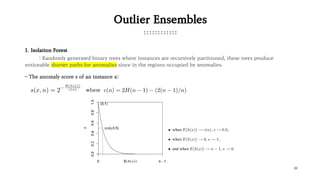
23. 23
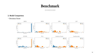
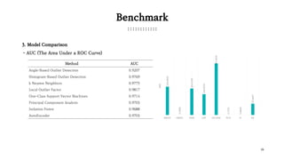
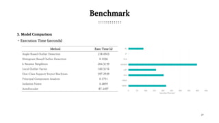
Benchmark
2. Model Selection
: Use model implemented in ‘pyod’ library. The parameters were selected through several tests.
Method Selected parameter (Others are default)
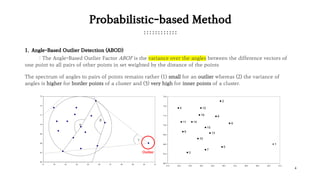
Angle-Based Outlier Detection {method=‘fast’}
Histogram-Based Outlier Detection {n_bins=5}
k Nearest Neighbors {n_neighbors=100}
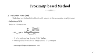
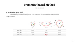
Local Outlier Factor {n_neighbors=300}
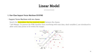
One-Class Support Vector Machines {kernel=‘rbf’}
Principal Component Analysis {}
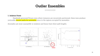
Isolation Forest {max_features=0.5, n_estimators=10, Bootstrap=False}
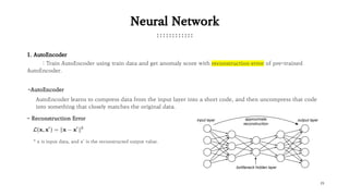
AutoEncoder
{hidden_neurons=[24, 16, 24], batch_size=2048,
epochs=300, validation_size=0.2}

24. 24
Benchmark
3. Model Comparison
- Decision Score
ABOD HBOS kNN
OCSVM PCA Isolation Forest AutoEncoder
LOF

25. 25
Benchmark
3. Model Comparison
- Precision-Recall curve (Baseline of Precision: 0.00159)
ABOD HBOS kNN LOF
OCSVM PCA Isolation Forest AutoEncoder

26. 26
Benchmark
3. Model Comparison
- AUC (The Area Under a ROC Curve)
218.4943
0.1036
204.3139
160.3154
397.2539
0.1751
0.4859
87.4497
ABOD HBOS KNN LOF OCSVM PCA IF AE
AUC
Method AUC
Angle-Based Outlier Detection 0.9207
Histogram-Based Outlier Detection 0.9769
k Nearest Neighbors 0.9775
Local Outlier Factor 0.9817
One-Class Support Vector Machines 0.9714
Principal Component Analysis 0.9703
Isolation Forest 0.9688
AutoEncoder 0.9703

27. 27
Benchmark
3. Model Comparison
- Execution Time (seconds)
0 50 100 150 200 250 300 350 400 450
ABOD
HBOS
Knn
LOF
OCSVM
PCA
IF
AE
Execution Time (sec)
Method Exec Time (s)
Angle-Based Outlier Detection 218.4943
Histogram-Based Outlier Detection 0.1036
k Nearest Neighbors 204.3139
Local Outlier Factor 160.3154
One-Class Support Vector Machines 397.2539
Principal Component Analysis 0.1751
Isolation Forest 0.4859
AutoEncoder 87.4497